|
|
|
|
|
|
|
|
In this article we try to explain to astrology students how to use basic statistical techniques to analyse astrological data. The methods belong to the standard statistical tools, taught at colleges and universities to present and analyse data for social and natural science. They can also be used to evaluate astrological data, as we will show you with a study that compares the astrological profiles of Art Critics with the expected values found in the Astrodienst database (ADB).
The goal of this article is not to present readers a case for or against astrology. Astrology as a science does not exist and for astrology as a belief system the rule ask one Jew, you'll get two opinions still applies. So you cannot simply test astrological claims, as there will always be astrologers who claim that the wrong test methods were used. This heterogeneity does not make astrology as such irrational, but it will make it difficult to test astrology empirically in an by astrologers or scientists accepted way. Statisticians and scientists are less interested in opinions. They want to present the data and analyze the data using standard methods that are based on proven mathematical formula's. What astrological findings are based on randomness and which outcomes could present a case for astrology?
Dane Rudhyar made some proposal to decipher this major astrological question in Statistical Astrology and Individuality, but his basic assumptions were rather naïve and speculative.
But Rudhyar, who criticized statistical testing as being too reductionistic, did not provide any objective tool to check his speculations about his “certainly not 100% accurate“ astrological prejudices. He ended his quest with circular reasoning:
For us, the simple goal was to find out what can astrologically be seen in the categories of the ADB database. Facts do matter and are more relevant to judges than the opinions of astrologers how things according their books or personal experience should be. Are there relevant astrological differences between ADB categories? Astrology books do assume them, but the only way to discover them is to simply compare ADB groups in a statistical way. For this reason we compared astrologically hundreds of ADB categories with the ADB as a whole. A list of them can be found here: ADB categories statistically evaluated.
The other goal of this article is to show our readers how easy it is to use statistical methods to do relevant astrological research. The tools are there, the time is right, and so the elemental astrological studies can and should be done.
We see no sound reasons for astrologers to postpone it.
Fifty years ago, researches needed access to expensive software like the Statistical Package for the Social Sciences (1968), but the basic statistical techniques can now be done by free open source software.
For centuries, astrologers used more or less precise ephemeris tables to calculate planet and house positions. But current astrology software calculates planet positions in milliseconds, presenting them in a pretty graphical way. Most astrology software can also do some research.
For centuries, astrological databases were unavailable. Astrology was explained by case studies, providing anecdotal evidence at best. Today, astrological databases are available on the internet, including plenty of biographical and other relevant data.
Actually, it should be a marvellous time to do predictive astrology again without relying on obscure and outdated astrological sources. As we have the tools and the data to identify the astrological risk factors for disease and disaster. Would you go back to the time when William Lilly presented his Christian astrology? Or the time when the disciples of Jesus presented their Gospels? Lilly, objective or not, became a hero for many astrologers. And Jesus, myth or not, became a God for the followers of his twelve apostles. But there are good reasons to doubt the validity of their mythical claims. For this reason new observations should be done, before maybe false gospels are endlessly repeated in time.
In the case of astrology, research can be redone using modern statistical techniques on the categories of the AstroDatabase (ADB). Of course, the study of astrology can still be done by doing private observations, but that would not make astrology a predictive science. It would stay a personal believe system, that somehow works for or appeals to some people, but has little predictive value for the rest.
The ADB was designed to enable astrological research, so it contains categories of groups that can be compared. See Help:Category - Astro-Databank for details.
The actual assignment of ADB entries to certain categories can often be disputed. Categories dealing with personality traits tend to be subjective, categories dealing with medical disease lack specificity. But what strikes most is the obvious underreporting in most categories: Why should only 53 ADB entries have an extraordinary talent for music in a database that contains at least famous 332 conductors, 1057 composers and 1976 instrumentalists?
The main reason for this obvious neglect is that the place, date and time of birth and especially the reliability of the birth time, have major priority of ADB editors. Here, and in the related concept of Rodden Rating they strive for scientific reliability and correct each other when needed, but the biography and categories are up to the preferences of the individual ADB editors. And because finding and documenting birth times is difficult enough, most ADB editors concentrate on this. Next, they add some categories that seem to be fitting to the record, some life events, and then they go on with the next record.
Only in exceptional cases, for instance when Louis Rodden described the faith of her family members or former ADB editor svi started his ADB rectification experiments, more attention to details were given in the ADB records. But most of the time ADB editors give only a short extract of facts as found in the Wikipedia. To copy and paste all of it to the ADB would be violation of the copyright. They assume that ADB users study the relevant Wikipedia entries to notice other biographical facts, including possible categories that could apply to the native.
So, if someone wants to study the astrology of anxiety disorder, looking only at the 48 cases mentioned in the ADB (0,1% of 50000) is a bad idea. As the sector Epidemiology of anxiety disorder of the Wikipedia suggests that there should be thousands of them (9 to 29% of the population).
This limitation of the ADB is not a public secret. In ADB Forums like Astro-Databank discussion, it has been explained. It is just a limitation dealing with priorities and lack of time of the ADB volunteers. Astrology researchers using the ADB categories should be aware of its limitations and try to correct for it, I read in 5.3. Data collection and submission of data to Astrodatabank:
Again, the priority of the ADB editors lies in the reliability of the found birth data. For this reason they prefer the often rounded Birth Certificate birth-time (Rodden rating AA), which can be imprecise, but is free from speculation. But other ADB claims tend to be hear say knowledge that come from several sources. So to do any serious research on ADB data the presented biographical data, presumed to be fitting categories and the many omissions in the tagged categories and personal data should also be checked, as one cannot expect that the few ADB editors have time to keep the large amount of biographical data updated. But of course the ADB editors did their best. And they had for sure no intention to deceive you by providing alternative facts. As they knew that facts can be checked. For this reason your and mine research of ADB categories like art critics can be fruitful. But it is important to know that in most categories not dealing with occupations, underreporting and thus systemic bias are rule.
AA times are the best Rodden Ratings to use in astrological research, as they are based on documented facts like the birth record, that can be checked. But few astrology students realise that a rounded 4 AM birth time could imply that the native could have a different ascendant, Moon sign and House Lords, when we see this AA time as having a imprecision of +/- 30 or even more minutes. And a shift in time of only 30 minutes would dramatically alter most predictive astrological techniques.
To deal with the rather imprecise given birth times of individuals, astrologers invented rectification techniques. But because those techniques can also be abused to explain wrong astrological theories afterwards with it, rectified times got a Rodden Rating of C (Caution, no source). So we only allowed them only in our control groups, where they could contribute their tiny part to the by statisticians and empirical scientists needed law of large numbers.
For statisticians studying astrology in large groups imprecise birth dates are a cause of extra noise in both their case and control groups. But statisticians studying the properties of large and small groups (samples) learned how to deal with noise in groups. As more or less imprecise measurements are always found. It causes more variation, especially in small groups. But estimations of the mean and likely variation around the found values can still be made.
But this on inherent uncertainty based error causes total unpredictability in groups consisting of one member, unless you study well-known matters like the theoretical question how many limbs a Sun in Aries had before he had his accidents. But the astrological assumption or as I assume astrological prejudices (bias) that people born with Sun in Aries are aggressive or are prone to accidents are “certainly not 100% accurate”.
Notwithstanding its limitations, the by Lois Rodden's initiated ADB database became a standard reference work most astrologers still do rely on. It is their best tool to demonstrate astrological principles when they strive for some objectivity. When astrologers always referred to their personal experience with anonymous private clients only, they would lose credibility. As that scientifically seen bad habit would make their unlikely claims impossible to check. So they prefer well known ADB entries to illustrate their point of view in astrology books, based on their personal experience over years with thousands of anonymous private clients and probably some hundreds astrology books. But makes this habit of paying selective attention you wise?
Astrologers seldom use case and control groups to do the kind of research that could give the astrological community answers to simple questions like: How more often are Sun in Taurus persons gardeners? What were the found and expected frequencies? Was the effect size large enough to be predictive in practice? Were the found differences statistically significant? Are the findings likely to be reproduced?
Without answering those basic questions, but only referring to private experiences and personal wisdom, astrology books will remain vague. To answer those questions, we did the work more bottom up. We did what David Cochrane called assumptionless research to avoid what the Wikipedia calls cherry-picking.
To accomplish this, we calculated of existing ADB Categories the found and the expected mean values of astrological parameters like planet in sign or house. That should be statistically seen all there is in the ADB. Then, we compared them using elementary statistical methods. For this, the so-called standard error had to be taken into account to answer the for predictive astrology important question: Are the found trends in the ADB categories likely to be reproduced? To answer those questions effect sizes and their confidence intervals had to be estimated. We developed some simple tools for this.
 In
this particular study we compare the astrological properties of
persons in the ADB category art critics with all timed ADB
entries of persons. But the methods also apply to the many other by
us investigated ADB categories. You can retrieve them all in
zipformat here.
In
this particular study we compare the astrological properties of
persons in the ADB category art critics with all timed ADB
entries of persons. But the methods also apply to the many other by
us investigated ADB categories. You can retrieve them all in
zipformat here.
The ADB as a whole could be seen as a sample of the population of all astrological charts, though it is certainly not a representative one. So we needed to provide you information about its major statistical characteristics. Not all control groups were done yet, but the selection criteria of TkDbAstro enables you to do most of the needed research yourselves. So you should not blame us as the messengers, but the missed opportunities you could do this job for your self. As the ADB is still the best source of birth time information of more or less known people that astrologers can access.
The only problem was that you had to study a lot of charts to do some research. And because it is impossible to oversee all those charts without making use of statistics, we developed a free tool for it. The credit for the programming goes to the in Switzerland born, Turkish geologist Tanberk Celalettin Kutlu, with the ADB Forum nickname of dildeolupbiten.
The painstaking work of arranging the selected raw astrological data from the AstroDatabase (ADB) to more informative statistical data presented in spreadsheets can be done by TkAstroDb. This open source Python program reads and processes the categorical data of ADB in contingency tables that can be read by well-known spreadsheets like Microsoft Excel and LibreOffice. You can retrieve the most recent results of the ADB Research Group in ADB stats.
In this article the focus is on the how, why and what to do with the by TkAstroDb provided statistical ADB data, using the principles of elemental statistical data analysis. We think that the frequencies found in the cross tables should be relevant for any genuine astrology researcher. As are the elemental statistical calculations done by TkAstroDb on expected values, effect-size, chi-square values, binomial p-values and (experimental) Cohen's d value. But of course, you are free to ignore them or understand them in your alternative way. We just provided the raw data that statisticians would like to see. See for my comments about the alternative views also Statistiek en astrologie volgens Dane Rudhyar (Dutch).
The installation and use TkAstroDb is explained at: http://github.com/dildeolupbiten/TkAstroDb.
TkAstroDb is still in development, so it is wise to check the above link for newer versions under Help /Check for updates.
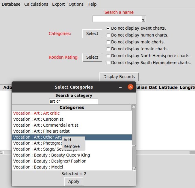
We observed the planet in sign and house positions of 79 persons categorised as Category:Vocation : Art : Art critic found in the extract of the Astrodienst database (ADB) of Nov, 28 2018 released at 23h09 or Adb_Version_181128_2309.
The inclusion criteria were: 1) Having the entry Vocation Art Critic in the ADB and 2) a Rodden rating of AA, A or B for the birth data.
The observed values of planet in sign and their standard deviations were:
|
Aries |
Taurus |
Gemini |
Cancer |
Leo |
Virgo |
Libra |
Scorpio |
Sag |
Cap |
Aqua |
Pisces |
SD |
|
|---|---|---|---|---|---|---|---|---|---|---|---|---|---|
|
Sun |
9 |
12 |
8 |
10 |
9 |
5 |
4 |
5 |
3 |
5 |
2 |
7 |
2,9 |
|
Moon |
6 |
9 |
5 |
4 |
9 |
8 |
8 |
2 |
7 |
8 |
9 |
4 |
2,3 |
|
Mercury |
9 |
8 |
11 |
6 |
10 |
4 |
3 |
7 |
4 |
3 |
5 |
9 |
2,7 |
|
Venus |
8 |
9 |
7 |
12 |
9 |
6 |
4 |
4 |
5 |
4 |
6 |
5 |
2,4 |
|
Mars |
10 |
6 |
4 |
9 |
4 |
11 |
5 |
8 |
6 |
8 |
3 |
5 |
2,5 |
|
Jupiter |
7 |
8 |
14 |
3 |
8 |
7 |
5 |
7 |
8 |
3 |
6 |
3 |
2,9 |
|
Saturn |
7 |
9 |
8 |
3 |
7 |
8 |
6 |
6 |
5 |
9 |
4 |
7 |
1,8 |
|
Uranus |
9 |
9 |
8 |
6 |
6 |
6 |
3 |
7 |
2 |
9 |
7 |
7 |
2,1 |
|
Neptune |
7 |
9 |
7 |
13 |
9 |
14 |
6 |
3 |
3 |
3 |
0 |
5 |
4,0 |
|
Pluto |
2 |
20 |
18 |
21 |
10 |
2 |
1 |
2 |
0 |
0 |
1 |
2 |
8,0 |
|
N Node |
9 |
11 |
4 |
4 |
6 |
4 |
5 |
9 |
4 |
6 |
5 |
12 |
2,8 |
|
Chiron |
14 |
15 |
2 |
5 |
5 |
2 |
5 |
1 |
1 |
4 |
11 |
14 |
5,2 |
|
Totals |
97 |
125 |
96 |
96 |
92 |
77 |
55 |
61 |
48 |
62 |
59 |
80 |
948 |
As you can see the observed difference between Sun in Taurus (12) and Sun in Aquarius (2) is quite large. Moon in Scorpio (2) scores low and Moon in Taurus (9) scores higher than expected. So there might be some astrological trends. Venus in cancer also scores 12, three times higher than the below average found values of Venus in Capricorn (4), Libra (4) and Scorpio (4). Of the personal planets Jupiter in Gemini (14) scores best.
An astrologer might comment: These findings do not surprise me, as Taureans love to be surrounded by beauty, but Aquarians behave more like a clochard. Aquarians do not attach to material things, but Taureans value them. These hindsight remarks sound reasonable. But would an astrologer be able to predict these tendencies before having access to the presented data? That is unlikely, as astrologers seldom publish any quantitative research.
Nevertheless, the qualitative explanation above could be a valid explanation for some interesting quantitative findings in this sample of art critics. Maybe other outcomes could be astrologically explained as well, so that some vague suggestions as found in astrology books, could become established facts found back in the ADB. But because of their initial vagueness (could instead of must), we would have not yet a case for astrology, as no clearly stated hypothesis was tested.
Statisticians would immediately notice the standard deviation (SD) presented in the last column. What does a SD of 2,9 imply for them? They would expect quite large deviations around the mean (79/12=6,6) with this small sample size. For them, knowing that the sample error plays a major role in producing variation, getting opposite results like Sun in Taurus (2) and Sun in Aquarius (12) could have happened just as well. Nevertheless, given the found data, they might predict that getting a Sun in Taurus would be more likely than getting a Sun in Aquarius with another sample of art critics. For the obvious reason that they have to adjust their chance models to the actual found data, not to the expected data. And they tend to change their views when the NULL hypothesis, predicting that the found values just reflected the expected variation found in a random ADB sample, would be rejected.
The positions of the house cusps and their standard deviations were:
|
Aries |
Taurus |
Gemini |
Cancer |
Leo |
Virgo |
Libra |
Scorpio |
Sag |
Cap |
Aqua |
Pisces |
SD |
|
|
Cusp 1 |
4 |
5 |
7 |
4 |
9 |
9 |
3 |
10 |
8 |
11 |
5 |
4 |
2,6 |
|
Cusp 2 |
7 |
4 |
9 |
6 |
5 |
8 |
9 |
2 |
10 |
3 |
12 |
4 |
3,0 |
|
Cusp 3 |
8 |
7 |
9 |
7 |
4 |
6 |
6 |
8 |
3 |
8 |
3 |
10 |
2,2 |
|
Cusp 4 |
8 |
10 |
9 |
8 |
6 |
4 |
6 |
6 |
8 |
4 |
5 |
5 |
1,9 |
|
Cusp 5 |
5 |
11 |
10 |
6 |
9 |
5 |
4 |
3 |
8 |
7 |
5 |
6 |
2,4 |
|
Cusp 6 |
7 |
5 |
15 |
10 |
2 |
6 |
6 |
3 |
4 |
8 |
8 |
5 |
3,3 |
|
Cusp 7 |
3 |
10 |
8 |
11 |
5 |
4 |
4 |
5 |
7 |
4 |
9 |
9 |
2,6 |
|
Cusp 8 |
9 |
2 |
10 |
3 |
12 |
4 |
7 |
4 |
9 |
6 |
5 |
8 |
3,0 |
|
Cusp 9 |
6 |
8 |
3 |
8 |
3 |
10 |
8 |
7 |
9 |
7 |
4 |
6 |
2,2 |
|
Cusp 10 |
6 |
6 |
8 |
4 |
5 |
5 |
8 |
10 |
9 |
8 |
6 |
4 |
1,9 |
|
Cusp 11 |
4 |
3 |
8 |
7 |
5 |
6 |
5 |
11 |
10 |
6 |
9 |
5 |
2,4 |
|
Cusp 12 |
6 |
3 |
4 |
8 |
8 |
5 |
7 |
5 |
15 |
10 |
2 |
6 |
3,3 |
The observed planets in Placidus houses and their standard deviations were:
|
H1 |
H2 |
H3 |
H4 |
H5 |
H6 |
H7 |
H8 |
H9 |
H10 |
H11 |
H12 |
SD |
|
|
Sun |
4 |
6 |
7 |
6 |
5 |
7 |
7 |
6 |
6 |
11 |
7 |
7 |
1,6 |
|
Moon |
10 |
8 |
8 |
6 |
4 |
10 |
5 |
7 |
10 |
2 |
5 |
4 |
2,6 |
|
Mercury |
5 |
4 |
6 |
7 |
7 |
7 |
4 |
9 |
8 |
10 |
5 |
7 |
1,8 |
|
Venus |
7 |
9 |
8 |
3 |
6 |
5 |
5 |
9 |
13 |
4 |
5 |
5 |
2,7 |
|
Mars |
6 |
6 |
3 |
2 |
7 |
7 |
11 |
12 |
6 |
5 |
10 |
4 |
3,0 |
|
Jupiter |
4 |
7 |
5 |
11 |
10 |
8 |
8 |
9 |
6 |
4 |
4 |
3 |
2,5 |
|
Saturn |
8 |
6 |
6 |
11 |
2 |
8 |
8 |
5 |
7 |
9 |
3 |
6 |
2,4 |
|
Uranus |
6 |
4 |
7 |
4 |
4 |
7 |
13 |
5 |
8 |
9 |
6 |
6 |
2,5 |
|
Neptune |
3 |
6 |
5 |
11 |
11 |
7 |
4 |
5 |
5 |
6 |
9 |
7 |
2,5 |
|
Pluto |
4 |
5 |
9 |
6 |
11 |
6 |
7 |
3 |
8 |
8 |
7 |
5 |
2,1 |
|
N Node |
6 |
10 |
2 |
6 |
5 |
6 |
5 |
7 |
12 |
6 |
7 |
7 |
2,4 |
|
Chiron |
9 |
6 |
9 |
5 |
3 |
4 |
11 |
10 |
3 |
7 |
6 |
6 |
2,6 |
When interpreting an individual chart, most astrologers would look for astrological indicators in the chart that matched with that profession. But what astrological factors are important for an art critic? How can they be known without having access to relevant empirical data?
Of course without relevant astrological data nothing special can be said. But astrological speculations can still be done. And the most appealing stories combine fact and fiction found in astrology books. The widely accepted practice among astrologers is to use their imagination to retell the found facts with the help of astrological symbolism. The applied symbols acts like a kind of glue that make their explanation look like astrology, just like the introduction of rhyme and metrics transforms a text into poetry.
Astrologers of course know that they cannot predict with the vague rules of astrological symbolism. Just like poets know that a well sounding poem still belongs to the realm of fiction. It is just their way of of story telling. But when astrologers can successfully frame their story with it astrological myths, it works for them and their clients, like well chosen political slogan can work for a campaign. See: Running for Office? Try These Political Campaign Slogan Ideas by Shane Daley. As politicians and astrologers want to convey a personal message, they are less interested in the facts.
Above we presented some major astrological properties of the category art critics from the ADB. Could they be used to interpret the chart of a person known to be an art critic? Could they predict a successful career in this field? To answer these questions one could do probability calculations on the astrological factors found the ADB group of art critics. Now the question is: Do we see certain patterns in it? And how should they be explained?
When interpreting ADB samples, including our ADB categories, astrologers and statisticians have different premises and points of views. What statisticians see as just another ADB sample probably showing the expected random values and bias, are for astrologers a group of unique individuals, whose essential individual properties one for one could linked to astrology.
Of course, not everything can be explained astrologically: Gender or homosexuality for instance cannot be read from a chart, but quite a lot could be explained when studying and combining enough astrological details, like We have a Sun in Taurus, having Lord 2 in 10, Venus in 9 etc. For this reason astrologers prefer to focus on individual charts, not on plain statistics that tend to blur the unique manifestation of each individual being or event. And here they have a point. Medical doctors and psychologists actually do the same.
See: The wisdom hierachy: A simple introduction to reasonable thinking.
Nevertheless, astrologers also deal with groups and risks, when they assume that people with a prominence of planets in Aries tend to be more aggressive. When astrologers see an aggressive individual having many planets in Aries, they would for sure recall that generalisation found in astrology books and see it as a case for astrology. And when not, another explanation had to be found. Empirical facts based on groups still do matter, and having a quick glance at the ADB category aggressive / brash could be wise.
But what is a “good enough” quick glance at this ADB category? Astrologers supposing that chance does not exist, systematically ignore the role that randomness plays in natural variability. For them, all they encounter is a kind of magic they like to play with it. Thus, the idea that getting 12 Taureans and only 2 Aquarians under 70 art critics could be due to some sampling error, would not impress them. As they dealt with real cases, not with statistical concepts. But a statistician could simply ask: What would happen if we had studied 790 instead of 79 cases of art critics? Would we still see those impressive patterns in the ADB? And a philosopher could ask: Are your astrological ideas also not concepts? Astrological concepts you project onto horoscopes, like tasseologists see them in the layout of tea leaves?
 Indeed,
our ADB observations could be the result of a well known bias that
has nothing to do with astrology as the study of significant
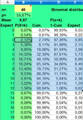
coincident patterns in the sky. When we throw 40 times a dice, we
will also see a large difference between the highest and lowest
value. Frequencies ranging from 2 to 12 would not be that unusual as
the Binomial distribution on the left predicts. Only the values 0, 1
and 13 or larger would be expected in less than 5% of cases.
Indeed,
our ADB observations could be the result of a well known bias that
has nothing to do with astrology as the study of significant
coincident patterns in the sky. When we throw 40 times a dice, we
will also see a large difference between the highest and lowest
value. Frequencies ranging from 2 to 12 would not be that unusual as
the Binomial distribution on the left predicts. Only the values 0, 1
and 13 or larger would be expected in less than 5% of cases.
Should we assume a false dice? Metaphysical factors? Jupiter in action? No, certainly not. It was just the sampling error. Some more throws are needed to infer that the dice is false or not. Only a fool would return to the shop to complain about a false dice after only forty trials with a dice.
For centuries layman, poets, theologians, mathematicians, polymaths, and astrologers speculated about risks and causality. They wrote books about the risks involved with eclipses, throwing a dice, offending the gods or having a bad or lucky day. And they also became interested in numbers. Is fasting 40 days enough to see something more? Numbers and relations between numbers (aspects) got significance.
In short: If you do this or see that, follows some another event after that quite more often? And when not, which other factors could be involved? That are still the major questions of all human and scientific thinking. But the ways to treat those questions differ a lot.
Today statistical tests are preferred to exclude coincidence, but few astrologers and even most scientists do not know that the first empirical definition of probability by Laplace, being the number of found cases divided by the number of possible cases, was not earlier formulated than in 1814. We now take his formula for granted, but before that risks dealt with deities. Fortune telling was seen as the work of special heavenly messengers and speculating about it was only the privilege of abstract thinking mathematicians and theologians. So, astrologers could ignore probability calculations for centuries. Astrologers saw the seven planets as gods ruling particular domains and were happy to be able to explain their world with it.
Actually, the confidence intervals involved with possible astrological effects were only calculated in the second halve of the 20th century. But since then the gap between the not using confidence intervals astrologers and scientists became huge. Applied scientists like medical doctors, sociologists and psychologists could profit enormously from statistical testing, but astrologers refused to see its benefits. See also: AstroWiki: Statistics: Continuing Controversy.
The by astrologers ignored rules of chance are just hidden in plain sight. As they always happen. But the same could be said of unusual coincidences. They also do happen. Only really blind persons could not see them. Astrologers expecting to encounter a meaningful cosmos instead of the usual chaos, prefer to link special life events with particular astrological events in the sky. They see any coincidence of them as an opportunity to explain their magical world to others, in which similar things seem to happen: As above, so below. But how could their found cases for astrology convince others? How could we reasonably check their assumptions?
Normally a theory is tested by its correct predictions. But the major problem with the unstructured approach of astrologers is that they can not (yet) predict with it. Using a myriad of vague, illogical and often contradictory rules, astrologers can explain almost everything, but when it comes to predicting facts one can not rely on fuzzy thinking. So, it is no coincidence that skilful astrologers showed up to be bad predictors in experimental tests.
In Sir Karl Popper' s vision the art of science is not just to explain events afterwards, but to predict them before they happened using the same strict empirical rules. For this reason Popper criticised the qualitative Marxist and Freudian theories as not being scientific. They could explain events afterwards, but could not be tested in practice. It is okay to conjecture a theory on the basis of historical events, but the theory should also be refutable. Scientific theories should be specific. Vague terms and concepts should be avoided.
Most scientists would agree with Popper that established facts do not need to be explained. And certainly not by unpredictive ad hoc methods used by astrologers, for the simple reason that you cannot explain things afterwards that you could not reasonably foresee. In their opinion, instead of providing hindsight wisdom that could lead to better attempts in the future, astrology as a pseudo-science would contribute to more Maya. Just like theologians did, when they explained human misery as God's punishment for personal sins.
Views that have little predictive value could be simply replied with a Is that so? or So what? When astrologers notice that you have a Pluto transit, you might accept that pseudo-astronomical reality with: So what? But it might affect you when you believed in astrology. Then the thinking error might refer to your attachment to astrology and your belief that a Pluto transit could influence your soul or ego, just like God is supposed to punish the sinners. In those situations of biased thinking placebo or nocebo effects could flourish just by suggestion. But that would still not be any proof of astrology or eternal justice being at at work. It would more likely be an instance of man's search for meaning, that science cannot provide.
Only when the same pattern repeatedly popped up much more than expected under believers and not believers, then there is a trend that needs further investigation. But we cannot rely on incidental observations and ad hoc rules, that sometimes confirm this principle, another time that rule, but in the long term would only give us false hope .
The immediately experienced unpredictability of many stochastic events contribute to the fun with gambling. This with the possibility of immediate gratification make dice games so addictive. This play with fortune will appeal even more to us when our life is rather dumb and boring. Do I become rich tonight in the casino with one more throw? Does Jupiter stands tonight favourable? That is the big roulette question. It could be the decisive moment people for years waited for.
This could be a good reason for you to watch your stars and numerology today. As chance does not exist according to their proponents. But there is also an inherent predictability when working with large numbers, where the business models of bookmakers and insurance companies rely on. They use statisticians to fill in this gap of uncertainty between immediate risks and long term effects by carefully estimating the risks of events that they could observe. They have a wait and see approach to by people shared suppositions without statistical proof. It would not influence their business as usual, unless this deviation from the found mean had some immediate marketing advantage for them.
But assuming that astrology can deal with this uncertainty for you seems rather foolish. Although some astrologers believed that they could explain the faith of lottery winners, they never became rich. Whatever method used, personal experience or scientific research, one can seldom predict new events with hindsight wisdom. That makes your life an empirical challenge.
But who is right? The individual gambler following his gut feeling in the here and now? Or statisticians and scientists dealing only with long term follow-up group behaviour? Actually, once established habits and presumptions predict most of the times the flow that people take. Even if it leads them probably in the wrong direction. How to predict this empirically found fact?
The practical problem is that we seldom have time and opportunity to do the necessary research. But we do have access to many opinions. The scientific approach can be boring, painstaking and will often be unavailable to most of us. And the scientific studies done might be irrelevant for the questions we are faced with. But we do have access to many opinions: On facebook, twitter ad the last breaking news.
Does this bombardment of news make you any wiser? No, as there is seldom a valid reason to assume that one point of view should win the contest. It could be more beneficial to accept the coexistence of different realms of reality that might enough complement each other. But that needs a lot training, as most born with views on the world, do differ a lot.
Statisticians do their claims on groups, never on individuals. But astrologers, psychologists and medical professionals deal with individuals. How could this work ever be done? It any rational prediction or explanation of the found facts possible, when their clients are always members of many astrological, psychological and medical categories at the same time? Their clients would thus to a certain extent follow a particular group rule, but few would be a typical exponent of that particular group, because the individual persons also belonged to quite different other groups and subcategorises.
One should not that easily generalise, but denying the existence of group effects would also be a mistake. As without clearly defined group effects, no sound medical or astrology book could ever be written. If all charts were unique and thus incomparable, there could not be any astro-logy at all. So, both medical doctors and astrologers should benefit from statistics comparing large groups. Well-designed prospective research on large groups is the cornerstone of evidence based medicine, on which most medical progress rest. Denying or neglecting its results could be a reason to suspend or ban a medical doctor. But in the world of astrology, the statistical empirical methods are met with suspicion if not with open hostility. But this has not been always been the case as the following history will tell you.
Between fun with dices and the law of the large numbers, there is a lot of room for speculation, the polymath Gerolamo Cardano found out (Wikipedia):
A logical and mathematical approach to the seven planets of astrology in the time of Cardano, is to assume that every planet has an equal risk of being placed in one of the twelve signs and houses. Then the risk of having Sun in sign or house could be calculated as 1/12. The risk of not falling into that sign would be calculated as 11/12. This is the binomial or p or p-1 approach of the usual this or that pertains kind of logical thinking.
When we found that plumbers had many more than expected (1/12) planets in scorpio, that would be called an astrological effect. See: The plumbers story .
But the problem is that we do not know the exact probability of any event in any group. So, assuming p is 1/12 seems to be a logical approach to deal with the astrological reality, but in empirical practice it is seldom correct. It is only a simple first best guess when dealing with fast moving personal planets in signs and houses. And it enables us to calculate the sampling error, which is important because it predicts which other values could be expected. From this we can estimate confidence intervals.
Actually, the risk involved with the houses is seldom 1/12, as all house systems have slow and fast rising signs. The inner planets Mercury and Venus do not move independently from the Sun, as they will always be close to the Sun. Statistical evaluation done with a control group could correct for many kinds of systemic thinking errors, but not for all. In this article we will show you several approaches.
 Binomial
calculator
Binomial
calculatorYou can download the spreadsheet which is used here as: Binomial_distribution_for_astrology.xlsx or Binomial_distribution_for_astrology.ods.
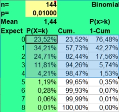
The binomial calculator used calculates the average frequency (mean) and the risks involved (P(X=k)) for found frequencies when throwing n times coins (p=1/2), dices (p=1/6) or doing astrological experiments with an assumed probability p = 1/12.
The risk of a hit is p and the risk of a miss is 1-p. This makes the distribution binomial, as only two possibilities (hit or miss) are investigated. A hit could be throwing a six with a dice (p = 1/6) or getting a Moon in Aries (p = 1/12), when investigating astrology. The risk of getting a frequency 0 to n hits for a particular side with n throws (experiments, cases) is displayed under the column P(X=k).
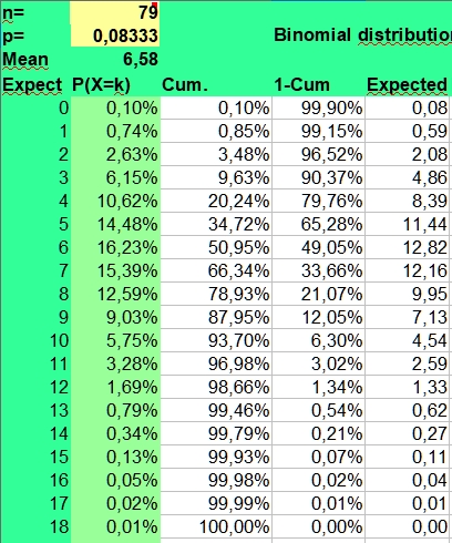
Under n (number) you fill in the number of investigated cases (here 79) and under p you fill in +1/12 to get the probability. The mean value is calculated as n*p or 79*1/12 = 6,58. But as the binomial distribution deals with discrete numbers, the values 6, 7 and 5 have the highest scores. Because of the asymmetry (skewness) of the distribution, 6 is more probable than the rounded mean 7 of 6,58. But as in the normal distributions, most values will fluctuate around the mean. Here values of 4 through 8 are found most often. They have a P(X=k)> 10% in the second column.
The spreadsheet also calculates Cumulative risks of getting a value of k or lower (third column) and the reverse risk 1- Cum of not getting a value of k or lower (fourth column), thus the risk of X > k (fourth column).
As you can see the risk of getting zero hits P(X = 0) for Sun in Aries with 79 throws of a fair 12 sided dice is only 0,10344 percent ((11/12)^79). Finding a frequency of zero cases for Sun in Aries is thus an unlikely event.
The expected value np of getting zero hits with 79 throws is 0,08 (79 times 0,0010), so when we would repeat this binomial experiment (n is 79, p = 1/12) a 100 times with fresh samples of 79, we could on average expect 8 cases of Sun in Aries having zero hits. Of course these 8 cases would be nothing compared to the most expected frequencies from 5 through 7 that would be seen more than a thousand times (100*12 is 1200).
But a point to remember is made. It is discussed under Data mining. When doing multiple observations, some unlikely findings are to be expected. In a crowded gambling hall there are always some excited winners. And that happy few could draw more attention than the expected majority of usual losers. Obviously this could lead to a false impression of what is going on or what statisticians call bias.
A low frequency of k = 2 has a binomial risk of 2,63%. Two cases could be expected, with a sample size of 79. So only the lower frequencies of 0 (0,10%) and 1 (0,74%) are within the exceptional 2,5% lower range of this binomial distribution.
The risk of getting the high frequency of k = 11 is 3,28%, which clearly falls outside the critical 2,5% upper range of a two-sided test. The risk of 12 is 1,69%, but values of 12 and higher are still found in 3,02% of cases. A frequency of 12 could be called borderline higher than expected, but not exceptionally high, as only frequencies above 12 are unlikely (1,34%) when applying common rules. Values from 2 through 12 could be expected in 98,66 - 0,85 = 97,81% of cases and values from 2 through 11 in 96,98 - 0,85 = 96,13% of cases. This is what we can expect assuming a risk of 1/12 and a sample size of 79.
Getting frequencies as low as of 2 or as high as 12, when 6 or 7 cases were expected, could hint to potential large effect sizes. But an astrological effect of a planet in sign or house must still be stronger, to reach statistical significance at the 5% level with 79 cases. As statistical significance depends strongly on sample size, much larger groups should be studied to see significant differences that could help us to come to conclusions. For this reason the statistician would ask, what if we studied 790 instead of 79 art critics?
In our study doing multiple measurements for planet in sign and house, every row yielding 12 values with a sum of 79 could wrongly be considered as containing 12 independent binomial tests with n is 79, p = 1/12. So, the measure of the 7 personal planets in sign, would yield 7 times 12 is 84 independent binomial tests. We might thus expect some 6 or 7 cases (84*0,10344) with a frequency of 0, but we did not encounter any zero at all.
For slow planets in sign zero frequencies were found and expected, but why did we not see them in the 144 measurements of planet in house? The reason is that we do not deal with a fair 12 sided dice , when dividing 79 possible hits over 12 signs and houses. Our situation is that of a sampling experiment without replacement. In that case the found frequencies per sign or house are not independent, as the sum of all values must equal the sample size. And then we may not use the multiplication rule of independent risks.
If you throw a fair dice, you will always get the same risk. New scores do not depend on previous ones. This is the situation of independent risks, the binomial distribution deals with. But when drawing lots, or when dividing 79 planets over 12 signs or houses, the calculations become much more complex as the possibilities of a new draw or assignment depend on the results of earlier throws.
Suppose that Sun in Aries had 19 hits against 79/12 (6,58) expected. This event with an effect size of 2,9 is very unlikely as P(x=19) = 0,0015% or 1 in 66894,3 cases and P(x>18) is 1 in 49048,7 cases. Then the expected value for having Sun in Taurus or another sign would be 60/11 (5,45). So the risk of getting another high score for the sun in another position would be much lower than the binomial distribution would have predicted. In this way there would be a kind of regression to the mean.
The same happens with the lower scores. If we had zero cases of Sun in Aries, the risk getting another low value in another sign would be very much decreased. As we now had to divide the 79 remaining hits over 11 instead of 12 signs. The expected value would be 79/11 (7,18) instead of 79/12 (6,58) of the binomial, which is 12/11 or 9,1 % higher.
So compared to the binomial distribution, when doing sampling experiments without replacement, clusters of extremely high or low values are not to be expected. High and low values are kept in balance as the sums of each row must be equal to the sample size.
Is that a major problem? Should we refrain from using the binomial distribution when calculating confidence intervals? No. The binomial distribution is still a great tool to predict the usual to be expected probabilities as the inaccuracies we speak of only happen with relatively small samples having extreme values (Outliers), like that of the ADB distribution of slow planets in sign. But here we often deal with special cases which cannot be explained with variance..
When dealing with larger samples, having smaller confidence intervals for the effect size, the calculated risks of the binomial distribution do in practice very well predict the actual values one could encounter. And the larger deviations only happen when the found values do differ a lot of the mean.
The risk of getting zero cases of Sun in Aries with a sample size of 790 would be extremely low, so low that you would not see it in practice (p = 1,40 E-30). But a similar unlikely event as getting P(X = 0) is 0,10344 % with 79 throws (Expected value is 0,08 or in practice most of the times zero) with a fair 12 sided dice is getting P (x=45) is 0,11% with a sample size of 790 (Expected value is 0,88, thus 1 case out of 790 expected). But here the error because of our sampling experiment without replacement would be less marked, as after getting an extremely low value of 45, the next 790 - 45 = 745 throws had to be divided over 11 instead of 12 signs. The expected value would be 745/11 (67,2) instead of the mean value 790/12 (65,8), which is only 2,8% higher. And that is a small deviation compared to the confidence interval of that estimate (50 - 81).
For statisticians regression to the mean refers to the empirical rule that the larger the sample taken from a population, the more closer the measured properties of that sample resemble the actual values of the studied population. But astrologers interpret statistical and empirical rules in an alternative way.
When Gauquelin's work on the Mars effect of medical doctors was redone with larger groups by a Belgian Committee, the found differences became less outspoken. Statisticians explained this as regression toward the mean. They concluded that Gauquelin's finding rested at least partly on the sampling error, that could be corrected for by taking larger samples. And when the effect size would be smaller with a large sample, there could be as well no effect at all.
Astrologers explained the less impressive results of the Belgian Committee by claiming that only Gauquelin's from the Who is who books selected professionals were iconic enough. The by the Belgians added not that famous medical doctors were just less special and thus would have a smaller Mars effect. So there would be an astrologically explainable reversion to mediocrity: Only the most celebrated types selected by Gauquelin would fully express the Mars effect and when adding many more mediocre professionals to the study group, their combined Mars and Jupiter effects would be less strong.
From the point of view of astrologers chance does not exist. At least not in the unique horoscopes they studied. So if a top ten of the greatest painters of the world would show certain patterns in their horoscopes, they would be regarded as typical of a genial painter. No control group and study of variation were needed, because there study group was unique. And when others did not see that pattern in the ADB category fine art artist (n = 1902), astrologers could simply explain away the discrepancy by stating that most of them were not that genial.
A statistician would say: You only studied 10 cases, while you should know that there are 12 signs for each planet! Imagine what would happen if we tested a dice with only 5 throws. You would at least miss one facet! And in your top 10 at least two and probably more possibilities are missed as P(x=0) is 41.9 % for p =1/12 and n=10 having an expected frequency of 3,49. This sample cannot be representative!
But the astrologer could majestically reply: We did not test a dice. Our selection was not random. We studied the top 10 painters and only them. So, the planets in sign we missed could not be typical of a genial artist. You can reproduce our experiment if you want with our selection. Then you would see that in our practice chance does not exist.
The unspoken premise and conclusion is that chance does not exist when we deal with unique events or samples. But applying this argumentation scheme to an indeed always changing reality is also a circle argument that cannot lead to any progress in astrology. For any astrology to be taken seriously, effect sizes do matter. And you cannot reasonably estimate and evaluate effect sizes and their confidence intervals without having some basic knowledge of statistics.
When an effective medical treatment against placebo is tested, we would expect more clear differences in effect size, the larger the sample size. Thus, with a larger sample size the initial effect size of 2,0 (+/- 0,5), could become 1,9 (+/- 0,2), but not 1,1 (+/- 0,2). See: The calculation of the effectiveness of medication.
In our opinion this methodology should also apply to presumed astrological effects. See: The relative risk of having an accident during a Mars conjunct Ascendant transit . When we compared small and large ADB categories with the ADB as a whole, the based on the sampling error regression to the mean rule clearly applies. The larger the categories, the smaller the effect sizes we encountered. And most statistically significant effect sizes were so small to predict with.
When studying many large tables as the ADB research group did (data-mining), there is similar sampling problem. If we do 100 tests with a significance level of 5%, on average five of them will just be significant by chance. They could be called false positive, as they suggest that something unusual is found, when actually nothing special happened.
If we only published the significant test results - suppose some 15 were found - there would be a publication bias in which on average 5 of the 15 test results could just be accidental findings. But the problem is that we can not reasonably know which results are due to chance and which are not.
 Actually
every observation will contain both elements, statistical noise and
real trends. So the variation caused by sampling errors can
hide small, but relevant effects, or exaggerate minimal trends, just
by chance. For this reason many more unbiased studies have to
be done and combined to see the real patterns, as just by
chance findings are unlikely to be repeated again. As only real
effects and systematic forms of bias do keep their patterns in time.
But biased observations do the same.
Actually
every observation will contain both elements, statistical noise and
real trends. So the variation caused by sampling errors can
hide small, but relevant effects, or exaggerate minimal trends, just
by chance. For this reason many more unbiased studies have to
be done and combined to see the real patterns, as just by
chance findings are unlikely to be repeated again. As only real
effects and systematic forms of bias do keep their patterns in time.
But biased observations do the same.
Is that error a reason to distrust statistics as many astrologers do? No. Professional astrologers also study and compare a lot of charts. But statisticians are aware of the statistical problems, estimate confidence intervals and can correct for multiple tests by decreasing the alpha.
So instead of stating in my experience plumbers have Mercury in Scorpio, one could better provide a more factual summary of the found data by stating: In one study of 12 plumbers, four of them had Mercury in Scorpio (p> 3 is = 0,014). See: The plumber's story for more details.
In our study 12x12 contingency tables with 144 found values are presented. With an alpha of 0,05 and 144 values, on average 7 extreme values per table could be found just by chance. If you fill in the binomial distribution with p = alpha and n= 144, you could see in the picture on the left that getting 3 up to 12 significantly lower or higher values per table would be quite normal (expected in 95% of the cases). And 13 would be borderline high value, as the risk of P>12 is 2,90%.
 For
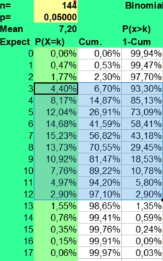
this reason most statisticians advise us to use a smaller alpha when
many values are compared. If we screened for unusual findings in a
12x12 table with an alpha of 0,01, much less false positives would be
found (mean 1, values above 4 being unlikely with a risk of 1,53%).
See the picture on the right.
For
this reason most statisticians advise us to use a smaller alpha when
many values are compared. If we screened for unusual findings in a
12x12 table with an alpha of 0,01, much less false positives would be
found (mean 1, values above 4 being unlikely with a risk of 1,53%).
See the picture on the right.
This statistical fact would be a good reason to use the mean +/- 2,58 sd values of the normal distribution in the binomial calculator as well. They give an indication of the to be expected 99% confidence interval. This approach yields much less statistical noise. When an astrological parameter is really predictive when interpreting charts, it should also pop up as being statically significant with a much smaller alpha.
Statisticians speak of the type 1 error when a true Null hypothesis is wrongly rejected. As we saw, the risk of this error depend on the chosen alpha. The larger the alpha, the larger the risk on false positives.
When doing one large and expensive experimental study testing the effectiveness of a medication against placebo, an alpha of 5% is quite acceptable. Because the reverse situation of rejecting a likely to be effective medicine because of lack of statistical significance (type 2 error) should be avoided. For this reason the required sample size to statistically proof the claimed effect size is calculated before the experiment is done.
But our study is not a well designed study to statistically proof any before the study started clearly expressed claim. We did not compare one particular study group with one well designed control group to watch the results (prospective study), but we compared all the ADB categories with the found values in the ADB as a whole (retrospective study). We studied ADB categories as they were found and compared them to the ADB as a whole (convenience sampling). In this case of doing hundreds of comparisons of found values against expected means, only extremely unlikely values should be regarded as significant. Would it be a problem that the alpha of 1 % would give many false negatives? No, and certainly not for predictive astrology as only large effect sizes could be predictive for that purpose
We described the statistical methods used to evaluate the data. And we invite you to try our methods out yourself using free software. Our simple approach was just to publish all of the in the ADB available data, if they fit current astrological opinions or not. But to evaluate them statistical methods are needed.
Quite a lot of astrological claims could be rejected with the found facts, thus with the ADB being statistically evaluated. But that was not our intention. We were just interested in the found facts. And we used statistical techniques to answer the relevant questions that any student of astrology would ask when being confronted many horoscopes. Could we predict with it? Could astrologers predict with it? And how well?
As a control group we used the ADB version exported on November, 28 2018 ( adb_export_181128_2309), our selection of art critics also came from . The statistical advantage is that we compared samples of the same population. The category art critics is just a subset of the ADB, so it should have similar statistical properties as the ADB as a whole. If the ADB is more or less normally distributed, its selected categories should be normally distributed as well. And that allows us to do statistical tests on found and expected values.
The inclusion criteria were having 1) a Rodden rating of AA, A, B or C for the birth data and 2) the entry should refer to the birth chart of a person.
This control group of 55047 ADB data of persons enabled us to calculate the expected planet positions using the formula X expected is 79/55047 times X observed in the control group.
The observed frequencies in the control group were:
|
Aries |
Taurus |
Gemini |
Cancer |
Leo |
Virgo |
Libra |
Scorpio |
Sag |
Cap |
Aqua |
Pisces |
Total |
|
|---|---|---|---|---|---|---|---|---|---|---|---|---|---|
|
Sun |
4738 |
4771 |
4772 |
4702 |
4731 |
4511 |
4522 |
4259 |
4194 |
4449 |
4601 |
4797 |
55047 |
|
Moon |
4673 |
4521 |
4652 |
4483 |
4618 |
4505 |
4538 |
4567 |
4576 |
4618 |
4652 |
4644 |
55047 |
|
Mercury |
4432 |
4299 |
4194 |
4184 |
4409 |
4584 |
4717 |
4823 |
4830 |
4828 |
4916 |
4831 |
55047 |
|
Venus |
4906 |
4787 |
4548 |
5134 |
4103 |
5243 |
3884 |
4579 |
4439 |
3890 |
5147 |
4387 |
55047 |
|
Mars |
3983 |
4332 |
4871 |
5128 |
5497 |
5489 |
5192 |
4802 |
4319 |
3912 |
3779 |
3743 |
55047 |
|
Jupiter |
4136 |
4224 |
4140 |
4597 |
4786 |
5150 |
5229 |
5146 |
4833 |
4441 |
4173 |
4192 |
55047 |
|
Saturn |
4125 |
4220 |
4249 |
4053 |
4559 |
4745 |
4836 |
4912 |
5139 |
5023 |
4822 |
4364 |
55047 |
|
Uranus |
5178 |
4924 |
6210 |
5130 |
4331 |
4187 |
4100 |
3673 |
3884 |
4159 |
3987 |
5284 |
55047 |
|
Neptune |
1854 |
2938 |
3608 |
5166 |
7319 |
8227 |
9330 |
6504 |
4489 |
2695 |
1495 |
1422 |
55047 |
|
Pluto |
1871 |
4484 |
9025 |
13318 |
12163 |
6223 |
3279 |
1949 |
778 |
462 |
342 |
1153 |
55047 |
|
N Node |
4739 |
4663 |
4911 |
4826 |
4615 |
4615 |
4591 |
4365 |
4302 |
4305 |
4487 |
4628 |
55047 |
|
Chiron |
9290 |
7520 |
4691 |
3276 |
2604 |
1884 |
2098 |
2618 |
2915 |
3864 |
6038 |
8249 |
55047 |
|
Aries |
Taurus |
Gemini |
Cancer |
Leo |
Virgo |
Libra |
Scorpio |
Sag |
Cap |
Aqua |
Pisces |
Total |
|
|
Cusp 1 |
2559 |
3199 |
4384 |
5542 |
6059 |
5956 |
6018 |
5838 |
5462 |
4236 |
3235 |
2559 |
55047 |
|
Cusp 2 |
3185 |
3646 |
4535 |
5403 |
5545 |
5363 |
5472 |
5605 |
5172 |
4540 |
3482 |
3099 |
55047 |
|
Cusp 3 |
3650 |
4119 |
4759 |
5192 |
5019 |
4917 |
4755 |
5161 |
5204 |
4599 |
4061 |
3611 |
55047 |
|
Cusp 4 |
4170 |
4468 |
5029 |
4962 |
4634 |
4192 |
4400 |
4495 |
5016 |
4974 |
4517 |
4190 |
55047 |
|
Cusp 5 |
4742 |
4947 |
5141 |
4650 |
4149 |
3788 |
3722 |
4103 |
4784 |
5118 |
5125 |
4778 |
55047 |
|
Cusp 6 |
5323 |
5481 |
5157 |
4581 |
3552 |
3219 |
3176 |
3642 |
4548 |
5407 |
5490 |
5471 |
55047 |
|
Cusp 7 |
6018 |
5838 |
5462 |
4236 |
3235 |
2559 |
2559 |
3199 |
4384 |
5542 |
6059 |
5956 |
55047 |
|
Cusp 8 |
5472 |
5605 |
5172 |
4540 |
3482 |
3099 |
3185 |
3646 |
4535 |
5403 |
5545 |
5363 |
55047 |
|
Cusp 9 |
4755 |
5161 |
5204 |
4599 |
4061 |
3611 |
3650 |
4119 |
4759 |
5192 |
5019 |
4917 |
55047 |
|
Cusp 10 |
4400 |
4495 |
5016 |
4974 |
4517 |
4190 |
4170 |
4468 |
5029 |
4962 |
4634 |
4192 |
55047 |
|
Cusp 11 |
3722 |
4103 |
4784 |
5118 |
5125 |
4778 |
4742 |
4947 |
5141 |
4650 |
4149 |
3788 |
55047 |
|
Cusp 12 |
3176 |
3642 |
4548 |
5407 |
5490 |
5471 |
5323 |
5481 |
5157 |
4581 |
3552 |
3219 |
55047 |
|
H1 |
H2 |
H3 |
H4 |
H5 |
H6 |
H7 |
H8 |
H9 |
H10 |
H11 |
H12 |
Total |
|
|
Sun |
5220 |
4975 |
4643 |
4287 |
4020 |
3961 |
4085 |
4141 |
4197 |
5072 |
5162 |
5284 |
55047 |
|
Moon |
4541 |
4557 |
4628 |
4567 |
4555 |
4554 |
4675 |
4493 |
4569 |
4579 |
4648 |
4681 |
55047 |
|
Mercury |
5187 |
5060 |
4808 |
4370 |
4100 |
4029 |
4053 |
3992 |
4448 |
4757 |
5036 |
5207 |
55047 |
|
Venus |
5124 |
4911 |
4656 |
4273 |
4220 |
4034 |
4080 |
4146 |
4463 |
4827 |
5096 |
5217 |
55047 |
|
Mars |
4732 |
4677 |
4523 |
4355 |
4400 |
4231 |
4454 |
4568 |
4554 |
4825 |
4802 |
4926 |
55047 |
|
Jupiter |
4529 |
4629 |
4657 |
4586 |
4663 |
4589 |
4499 |
4496 |
4538 |
4731 |
4481 |
4649 |
55047 |
|
Saturn |
4696 |
4650 |
4526 |
4680 |
4619 |
4622 |
4633 |
4467 |
4412 |
4481 |
4603 |
4658 |
55047 |
|
Uranus |
4580 |
4421 |
4436 |
4477 |
4561 |
4472 |
4664 |
4632 |
4779 |
4678 |
4776 |
4571 |
55047 |
|
Neptune |
4530 |
4517 |
4463 |
4483 |
4582 |
4496 |
4577 |
4756 |
4794 |
4582 |
4648 |
4619 |
55047 |
|
Pluto |
3871 |
3757 |
3993 |
3951 |
3853 |
3866 |
5217 |
5231 |
5327 |
5273 |
5417 |
5291 |
55047 |
|
N Node |
4520 |
4525 |
4505 |
4536 |
4717 |
4603 |
4528 |
4535 |
4679 |
4603 |
4627 |
4669 |
55047 |
|
Chiron |
4541 |
4553 |
4464 |
4566 |
4656 |
4564 |
4624 |
4538 |
4652 |
4669 |
4579 |
4641 |
55047 |
 The
control group is large enough to test some assumptions using the
normal distribution. Are the planets evenly distributed in
sign?
The
control group is large enough to test some assumptions using the
normal distribution. Are the planets evenly distributed in
sign?
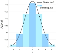
We could make use of the empirical statistical rule, that states that if the sample size is large enough, the shapes of the discrete binomial distribution and the continuous normal distribution will be similar. This will be most apparent with coin tossing (p =0,5), as shown in the picture on the right taken from the Wikipedia, because then we do not see any skewness in the binomial distribution. But when the expected value np > 10 and n(1-p) are larger than 10 the similarity rule applies. Less strict criteria use np > 5.
Translated to the astrological practice with p = 1/12, sample sizes of selected ADB categories should be in the order of 120 (60) or higher to expect roughly a normal distribution for the values of the observed frequencies. But is that enough to show astrological effects in a statistical way?
Let us go on with the interpretation of numbers like statisticians do, and apply the above mathematical considerations to astrological data. If the planets in sign are evenly distributed, then the found frequencies should be near the expected value np (mean) in terms of standard deviations. The standard deviation can be estimated as the square root of variance np(1-p) of the binomial distribution when np is large enough (preferably > 10, but > 5 might do).
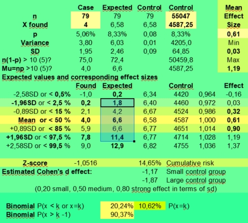
The spreadsheet which we use to calculate these expected frequencies is again : Binomial_distribution_for_astrology.xlsx or Binomial_distribution_for_astrology.ods. On the right it contains a simple calculator where you can fill in the numbers found and expected for the case and control groups and their sample sizes (yellow area). Then it will calculate the expected probability p for the case and control groups, the variance and standard deviations, some parameters like n(1-p) and np and most important for our purpose the Expected frequencies and corresponding effect sizes.
 When
the control groups consists of n = 55047 persons, then the mean value
with p is 1/12 is 4587,25 and the expected standard deviation would
be 64,8. See the upper values in 5th column.
When
the control groups consists of n = 55047 persons, then the mean value
with p is 1/12 is 4587,25 and the expected standard deviation would
be 64,8. See the upper values in 5th column.
According to statisticians 70 % of the values should fall in the np +/- 0,89 SD range of 4524 - 4651 and circa 95% of the values in the np +/- 1,96 SD range of 4460 - 4714.
In the large control group, some 70 % of observed frequencies would vary only 1,4 % around the mean (effect sizes of 0,986 - 1,014) and some 95% of expected frequencies would vary at most 2,8 % around the mean (effect sizes of 0,972 - 1,028).
So tiny effect sizes of +/ - 2,9 % or more could be statistical significant with a sample size of 55047, p is 1/12 and an alpha of 0,05. If you would use an alpha of 0,01 effect sizes of 3,7 % or larger were needed (sixth lower column gives a range of 0,964 - 1,036).
But a found effect size of 0,61 (39 % less) with k is 4 against 6,58 expected for the small case group with n is 79, has a wide range of not significant effect sizes if the sampling error is taken into account: 0,03 - 1,19 (upper right in the calculator). Only found values of 0, 1 and 12 and higher would fall outside the expected 95% confidence interval of 1,8 - 11,4 (third column) of values that in 95% of samples just could have been arisen by chance.
And if we would use an alpha of 1 % to compensate for our data mining, only values above 12,9 having an effect size of 1,83 or more would be significant, and the rest just could be discarded as being a likely result of the sampling error.
When you would fill in X found is 40 with n is 790, the range of estimated effect sizes would still be 0,42 - 0,79 (95 %) with an expected value of 65,8 (50,6 - 81,1). With X is 120 and n is 790 as in the Sun in Taurus case, the effect size range is 1,52 - 2,12 (95 %), but with k is 12 and n =79 having Sun in taurus could have both positive or negative effects with an expected effect size range from 0,87 to 2,77. It is actually 0,84 - 2,67 when using the found value 4771 for Sun in Taurus of the control group instead of the expected value of +55047/12.
So you see that both the exact approach using the binomial calculator as the normal distribution approach for this problem produce similar results. In both cases we had to conclude that a value of 12 found against 6,58 expected (mean effect size 1,75) was not significant enough to provide evidence of a positive effect given the small sample size of 79. It could be a real positive effect that would be repeated again when doing more research, but this assumption still has to be proven.
Is the ADB evenly distributed? No, certainly not. This is most evident for slow planets in sign, but it also applies to the personal planets with the exception of the fast moving moon. The found frequencies deviate more from the mean than we expected. With p is 1/12 and n is 55047 we expect values that deviated only ± 1% (± 1sd) from the mean in 70% of cases or ± 3% (± 2 sd) from the mean in 95% of cases, but as you can see the lowest frequency of 4194 for Sun in Sagittarius in the control group is 91% of the expected value. The highest value for sun sign Pisces (4797) is 105% of the mean. The actual standard deviations found in the rows are shown in the last column in the table below.
|
Aries |
Taurus |
Gemini |
Cancer |
Leo |
Virgo |
Libra |
Scorpio |
Sag |
Cap |
Aqua |
Pisces |
SD |
|
|---|---|---|---|---|---|---|---|---|---|---|---|---|---|
|
Sun |
4738 |
4771 |
4772 |
4702 |
4731 |
4511 |
4522 |
4259 |
4194 |
4449 |
4601 |
4797 |
195,8 |
|
Moon |
4673 |
4521 |
4652 |
4483 |
4618 |
4505 |
4538 |
4567 |
4576 |
4618 |
4652 |
4644 |
61,8 |
|
Mercury |
4432 |
4299 |
4194 |
4184 |
4409 |
4584 |
4717 |
4823 |
4830 |
4828 |
4916 |
4831 |
260,3 |
|
Venus |
4906 |
4787 |
4548 |
5134 |
4103 |
5243 |
3884 |
4579 |
4439 |
3890 |
5147 |
4387 |
453,0 |
|
Mars |
3983 |
4332 |
4871 |
5128 |
5497 |
5489 |
5192 |
4802 |
4319 |
3912 |
3779 |
3743 |
629,1 |
|
Jupiter |
4136 |
4224 |
4140 |
4597 |
4786 |
5150 |
5229 |
5146 |
4833 |
4441 |
4173 |
4192 |
410,8 |
|
Saturn |
4125 |
4220 |
4249 |
4053 |
4559 |
4745 |
4836 |
4912 |
5139 |
5023 |
4822 |
4364 |
358,3 |
|
Uranus |
5178 |
4924 |
6210 |
5130 |
4331 |
4187 |
4100 |
3673 |
3884 |
4159 |
3987 |
5284 |
719,6 |
|
Neptune |
1854 |
2938 |
3608 |
5166 |
7319 |
8227 |
9330 |
6504 |
4489 |
2695 |
1495 |
1422 |
2606,6 |
|
Pluto |
1871 |
4484 |
9025 |
13318 |
12163 |
6223 |
3279 |
1949 |
778 |
462 |
342 |
1153 |
4410,1 |
|
N Node |
4739 |
4663 |
4911 |
4826 |
4615 |
4615 |
4591 |
4365 |
4302 |
4305 |
4487 |
4628 |
185,8 |
|
Chiron |
9290 |
7520 |
4691 |
3276 |
2604 |
1884 |
2098 |
2618 |
2915 |
3864 |
6038 |
8249 |
2459,6 |
Clearly, the planets in the large ADB control group are not evenly distributed in sign. The slower the planet as seen from the earth is moving, the less even is its distribution in the ADB. And the higher the standard deviations become.
If we express the found values in terms of expected standard deviations away from the mean, thus (x-np) / sd or (x-55047/12) / 64,85, we see again that only the values of the fast moving moon fall within the expected mean +/- 2 sd range.
|
Aries |
Taurus |
Gemini |
Cancer |
Leo |
Virgo |
Libra |
Scorpio |
Sag |
Cap |
Aqua |
Pisces |
|
|---|---|---|---|---|---|---|---|---|---|---|---|---|
|
Sun |
2,32 |
2,83 |
2,85 |
1,77 |
2,22 |
-1,18 |
-1,01 |
-5,06 |
-6,06 |
-2,13 |
0,21 |
3,23 |
|
Moon |
1,32 |
-1,02 |
1,00 |
-1,61 |
0,47 |
-1,27 |
-0,76 |
-0,31 |
-0,17 |
0,47 |
1,00 |
0,88 |
|
Mercury |
-2,39 |
-4,45 |
-6,06 |
-6,22 |
-2,75 |
-0,05 |
2,00 |
3,64 |
3,74 |
3,71 |
5,07 |
3,76 |
|
Venus |
4,92 |
3,08 |
-0,61 |
8,43 |
-7,47 |
10,11 |
-10,84 |
-0,13 |
-2,29 |
-10,75 |
8,63 |
-3,09 |
|
Mars |
-9,32 |
-3,94 |
4,38 |
8,34 |
14,03 |
13,91 |
9,33 |
3,31 |
-4,14 |
-10,41 |
-12,46 |
-13,02 |
|
Jupiter |
-6,96 |
-5,60 |
-6,90 |
0,15 |
3,06 |
8,68 |
9,90 |
8,62 |
3,79 |
-2,26 |
-6,39 |
-6,10 |
|
Saturn |
-7,13 |
-5,66 |
-5,22 |
-8,24 |
-0,44 |
2,43 |
3,84 |
5,01 |
8,51 |
6,72 |
3,62 |
-3,44 |
|
Uranus |
9,11 |
5,19 |
25,02 |
8,37 |
-3,95 |
-6,17 |
-7,51 |
-14,10 |
-10,84 |
-6,60 |
-9,26 |
10,74 |
|
Neptune |
-42,15 |
-25,43 |
-15,10 |
8,93 |
42,13 |
56,13 |
73,14 |
29,56 |
-1,52 |
-29,18 |
-47,69 |
-48,81 |
|
Pluto |
-41,89 |
-1,59 |
68,44 |
134,64 |
116,83 |
25,23 |
-20,17 |
-40,68 |
-58,74 |
-63,62 |
-65,47 |
-52,96 |
|
N Node |
2,34 |
1,17 |
4,99 |
3,68 |
0,43 |
0,43 |
0,06 |
-3,43 |
-4,40 |
-4,35 |
-1,55 |
0,63 |
|
Chiron |
72,52 |
45,23 |
1,60 |
-20,22 |
-30,58 |
-41,69 |
-38,39 |
-30,37 |
-25,79 |
-11,15 |
22,37 |
56,47 |
The found standard deviation 61,8 for moon in sign (see above), comes close to the calculated SD of 64,85. But the found standard deviation of Pluto in sign of 4410 is 68 times larger. Of course the very uneven distribution for outer planets in sign could be expected. For historical reasons the ADB is unevenly distributed in time. But the variations for Sun in sign and the inner planets were also larger than we expected. Only the moon seems to move fast enough to create the expected randomness.
These discrepancies between expected and found values do not plead against doing statistics with the ADB. It only reinforces our opinion that cautiousness, control groups and statistical techniques are needed when doing astrological research, as we cannot rely on naive astronomical assumptions. But we certainly can not rely on even more naive astrological assumptions found in astrology books and Forums.
The expected planet positions were calculated as x expected is 79/55047 times x observed in the control group.
|
Aries |
Taurus |
Gemini |
Cancer |
Leo |
Virgo |
Libra |
Scorpio |
Sag |
Cap |
Aqua |
Pisces |
Total |
|
|---|---|---|---|---|---|---|---|---|---|---|---|---|---|
|
Sun |
6,80 |
6,85 |
6,85 |
6,75 |
6,79 |
6,47 |
6,49 |
6,11 |
6,02 |
6,38 |
6,60 |
6,88 |
79,00 |
|
Moon |
6,71 |
6,49 |
6,68 |
6,43 |
6,63 |
6,47 |
6,51 |
6,55 |
6,57 |
6,63 |
6,68 |
6,66 |
79,00 |
|
Mercury |
6,36 |
6,17 |
6,02 |
6,00 |
6,33 |
6,58 |
6,77 |
6,92 |
6,93 |
6,93 |
7,06 |
6,93 |
79,00 |
|
Venus |
7,04 |
6,87 |
6,53 |
7,37 |
5,89 |
7,52 |
5,57 |
6,57 |
6,37 |
5,58 |
7,39 |
6,30 |
79,00 |
|
Mars |
5,72 |
6,22 |
6,99 |
7,36 |
7,89 |
7,88 |
7,45 |
6,89 |
6,20 |
5,61 |
5,42 |
5,37 |
79,00 |
|
Jupiter |
5,94 |
6,06 |
5,94 |
6,60 |
6,87 |
7,39 |
7,50 |
7,39 |
6,94 |
6,37 |
5,99 |
6,02 |
79,00 |
|
Saturn |
5,92 |
6,06 |
6,10 |
5,82 |
6,54 |
6,81 |
6,94 |
7,05 |
7,38 |
7,21 |
6,92 |
6,26 |
79,00 |
|
Uranus |
7,43 |
7,07 |
8,91 |
7,36 |
6,22 |
6,01 |
5,88 |
5,27 |
5,57 |
5,97 |
5,72 |
7,58 |
79,00 |
|
Neptune |
2,66 |
4,22 |
5,18 |
7,41 |
10,50 |
11,81 |
13,39 |
9,33 |
6,44 |
3,87 |
2,15 |
2,04 |
79,00 |
|
Pluto |
2,69 |
6,44 |
12,95 |
19,11 |
17,46 |
8,93 |
4,71 |
2,80 |
1,12 |
0,66 |
0,49 |
1,65 |
79,00 |
|
N Node |
6,80 |
6,69 |
7,05 |
6,93 |
6,62 |
6,62 |
6,59 |
6,26 |
6,17 |
6,18 |
6,44 |
6,64 |
79,00 |
|
Chiron |
13,33 |
10,79 |
6,73 |
4,70 |
3,74 |
2,70 |
3,01 |
3,76 |
4,18 |
5,55 |
8,67 |
11,84 |
79,00 |
As we have seen the values for sun and moon sign were not exactly 79/12 is 6,58 in the ADB. Nevertheless for sun and moon sign, expecting values around 6 and 7 seems reasonable. For most personal planets values between 5 and 8 could be expected.
But for slow planets and points there is much more variation, due to the unequal distribution of the ADB entries in time, with entries of the 19th and 20th centuries prevailing. The ADB preference of entering persons with a timed birth record (BC) resulted in an over-representation of entries from particular Western countries, where the birth-time was recorded in the birth certificate from the early 18th century onwards. This not by randomness nor astrological factors determined variation makes the statistical and astrological interpretation of the slow planets in sign difficult. Astrologers are aware of this problem and speak of generational factors when interpreting slow planets in sign in individual charts.
One could try to fix it with artificially generated control groups that lived in a similar time, but before fixing any error one should thoroughly understand the nature of the problem one wants to correct for. It is an historical fact that punks, dadaists and romantic poets lived in different times. Are they astrologically seen similar? Maybe. But in this case trying to correct for the Zeitgeist, without understanding its nature, could be throwing the baby out with the bathwater. Maybe relevant aspects between personal planets and slow planets would be thrown away as well.
The impact of a slow or fast rising sign is large. In the Northern hemisphere, Aries and Pisces are the fast rising signs. As you can see below, you will twice more often encounter someone with Ascendant in Cancer to Sagittarius, than Ascendant in Aries or Pisces. So when studying astrological houses, we have to take into account the distribution of the declinations in case and control groups.
|
Aries |
Taurus |
Gemini |
Cancer |
Leo |
Virgo |
Libra |
Scorpio |
Sag |
Cap |
Aqua |
Pisces |
Total |
|
|---|---|---|---|---|---|---|---|---|---|---|---|---|---|
|
Cusp 1 |
3,67 |
4,59 |
6,29 |
7,95 |
8,70 |
8,55 |
8,64 |
8,38 |
7,84 |
6,08 |
4,64 |
3,67 |
79,00 |
|
Cusp 2 |
4,57 |
5,23 |
6,51 |
7,75 |
7,96 |
7,70 |
7,85 |
8,04 |
7,42 |
6,52 |
5,00 |
4,45 |
79,00 |
|
Cusp 3 |
5,24 |
5,91 |
6,83 |
7,45 |
7,20 |
7,06 |
6,82 |
7,41 |
7,47 |
6,60 |
5,83 |
5,18 |
79,00 |
|
Cusp 4 |
5,98 |
6,41 |
7,22 |
7,12 |
6,65 |
6,02 |
6,31 |
6,45 |
7,20 |
7,14 |
6,48 |
6,01 |
79,00 |
|
Cusp 5 |
6,81 |
7,10 |
7,38 |
6,67 |
5,95 |
5,44 |
5,34 |
5,89 |
6,87 |
7,35 |
7,36 |
6,86 |
79,00 |
|
Cusp 6 |
7,64 |
7,87 |
7,40 |
6,57 |
5,10 |
4,62 |
4,56 |
5,23 |
6,53 |
7,76 |
7,88 |
7,85 |
79,00 |
|
Cusp 7 |
8,64 |
8,38 |
7,84 |
6,08 |
4,64 |
3,67 |
3,67 |
4,59 |
6,29 |
7,95 |
8,70 |
8,55 |
79,00 |
|
Cusp 8 |
7,85 |
8,04 |
7,42 |
6,52 |
5,00 |
4,45 |
4,57 |
5,23 |
6,51 |
7,75 |
7,96 |
7,70 |
79,00 |
|
Cusp 9 |
6,82 |
7,41 |
7,47 |
6,60 |
5,83 |
5,18 |
5,24 |
5,91 |
6,83 |
7,45 |
7,20 |
7,06 |
79,00 |
|
Cusp 10 |
6,31 |
6,45 |
7,20 |
7,14 |
6,48 |
6,01 |
5,98 |
6,41 |
7,22 |
7,12 |
6,65 |
6,02 |
79,00 |
|
Cusp 11 |
5,34 |
5,89 |
6,87 |
7,35 |
7,36 |
6,86 |
6,81 |
7,10 |
7,38 |
6,67 |
5,95 |
5,44 |
79,00 |
|
Cusp 12 |
4,56 |
5,23 |
6,53 |
7,76 |
7,88 |
7,85 |
7,64 |
7,87 |
7,40 |
6,57 |
5,10 |
4,62 |
79,00 |
As most of the ADB entries were born in the Northern Hemisphere, the fast rising Aries and Pisces ascendants were underrepresented in our control group. Of course Aries and Pisces score high on the descendant.
Looking at the standard deviations of the Placidus house cusp in sign distribution of the 55047 entries of the control group, we see that they are largest on the 1-7 axis and lowest on the 4-10 axis.
|
Aries |
Taurus |
Gemini |
Cancer |
Leo |
Virgo |
Libra |
Scorpio |
Sag |
Cap |
Aqua |
Pisces |
SD |
|
|---|---|---|---|---|---|---|---|---|---|---|---|---|---|
|
Cusp 1 |
2559 |
3199 |
4384 |
5542 |
6059 |
5956 |
6018 |
5838 |
5462 |
4236 |
3235 |
2559 |
1337,8 |
|
Cusp 2 |
3185 |
3646 |
4535 |
5403 |
5545 |
5363 |
5472 |
5605 |
5172 |
4540 |
3482 |
3099 |
941,6 |
|
Cusp 3 |
3650 |
4119 |
4759 |
5192 |
5019 |
4917 |
4755 |
5161 |
5204 |
4599 |
4061 |
3611 |
559,5 |
|
Cusp 4 |
4170 |
4468 |
5029 |
4962 |
4634 |
4192 |
4400 |
4495 |
5016 |
4974 |
4517 |
4190 |
319,1 |
|
Cusp 5 |
4742 |
4947 |
5141 |
4650 |
4149 |
3788 |
3722 |
4103 |
4784 |
5118 |
5125 |
4778 |
493,6 |
|
Cusp 6 |
5323 |
5481 |
5157 |
4581 |
3552 |
3219 |
3176 |
3642 |
4548 |
5407 |
5490 |
5471 |
902,0 |
|
Cusp 7 |
6018 |
5838 |
5462 |
4236 |
3235 |
2559 |
2559 |
3199 |
4384 |
5542 |
6059 |
5956 |
1337,8 |
|
Cusp 8 |
5472 |
5605 |
5172 |
4540 |
3482 |
3099 |
3185 |
3646 |
4535 |
5403 |
5545 |
5363 |
941,6 |
|
Cusp 9 |
4755 |
5161 |
5204 |
4599 |
4061 |
3611 |
3650 |
4119 |
4759 |
5192 |
5019 |
4917 |
559,5 |
|
Cusp 10 |
4400 |
4495 |
5016 |
4974 |
4517 |
4190 |
4170 |
4468 |
5029 |
4962 |
4634 |
4192 |
319,1 |
|
Cusp 11 |
3722 |
4103 |
4784 |
5118 |
5125 |
4778 |
4742 |
4947 |
5141 |
4650 |
4149 |
3788 |
493,6 |
|
Cusp 12 |
3176 |
3642 |
4548 |
5407 |
5490 |
5471 |
5323 |
5481 |
5157 |
4581 |
3552 |
3219 |
902,0 |
No standard deviation comes close to the expected standard deviation for a binomial distribution with n= 55047 and p =1/2 being the square root of variance np(1-p) =64,85. But that would not be a surprise if you knew that the Placidus house system does not equally distribute houses along the Western zodiac.
When looking at the distribution of the planet in the Placidus houses of the control group (n = 55047 ), we see that the standard deviations for the Sun (501), Mercury (457), Venus (420), Mars (201), and Pluto (709) are much higher than expected (65).
|
H1 |
H2 |
H3 |
H4 |
H5 |
H6 |
H7 |
H8 |
H9 |
H10 |
H11 |
H12 |
SD |
|
|---|---|---|---|---|---|---|---|---|---|---|---|---|---|
|
Sun |
5220 |
4975 |
4643 |
4287 |
4020 |
3961 |
4085 |
4141 |
4197 |
5072 |
5162 |
5284 |
501,0 |
|
Moon |
4541 |
4557 |
4628 |
4567 |
4555 |
4554 |
4675 |
4493 |
4569 |
4579 |
4648 |
4681 |
55,3 |
|
Mercury |
5187 |
5060 |
4808 |
4370 |
4100 |
4029 |
4053 |
3992 |
4448 |
4757 |
5036 |
5207 |
456,6 |
|
Venus |
5124 |
4911 |
4656 |
4273 |
4220 |
4034 |
4080 |
4146 |
4463 |
4827 |
5096 |
5217 |
420,1 |
|
Mars |
4732 |
4677 |
4523 |
4355 |
4400 |
4231 |
4454 |
4568 |
4554 |
4825 |
4802 |
4926 |
201,2 |
|
Jupiter |
4529 |
4629 |
4657 |
4586 |
4663 |
4589 |
4499 |
4496 |
4538 |
4731 |
4481 |
4649 |
76,4 |
|
Saturn |
4696 |
4650 |
4526 |
4680 |
4619 |
4622 |
4633 |
4467 |
4412 |
4481 |
4603 |
4658 |
88,6 |
|
Uranus |
4580 |
4421 |
4436 |
4477 |
4561 |
4472 |
4664 |
4632 |
4779 |
4678 |
4776 |
4571 |
117,4 |
|
Neptune |
4530 |
4517 |
4463 |
4483 |
4582 |
4496 |
4577 |
4756 |
4794 |
4582 |
4648 |
4619 |
99,6 |
|
Pluto |
3871 |
3757 |
3993 |
3951 |
3853 |
3866 |
5217 |
5231 |
5327 |
5273 |
5417 |
5291 |
709,0 |
|
N Node |
4520 |
4525 |
4505 |
4536 |
4717 |
4603 |
4528 |
4535 |
4679 |
4603 |
4627 |
4669 |
69,5 |
|
Chiron |
4541 |
4553 |
4464 |
4566 |
4656 |
4564 |
4624 |
4538 |
4652 |
4669 |
4579 |
4641 |
59,0 |
In the case of the Sun, the left hemisphere seems to be preferred, the peak position being the 12th house (5284) and the lowest value in the 6th house (3961). Mercury and Venus, always in the neighbourhood of the Sun, follow this tendency. The effect is also seen with Mars, which reminds us of the Mars effect. In the case of Pluto, the most striking finding is that 23291 (42,3%) entries are below and 31756 (57,7%) entries are above the horizon.
The above tendencies can be more clearly seen, when we calculate the value (x found - mean) divided by the standard deviation of that row.
|
Placidus |
H1 |
H2 |
H3 |
H4 |
H5 |
H6 |
H7 |
H8 |
H9 |
H10 |
H11 |
H12 |
SD |
|
Sun |
1,26 |
0,77 |
0,11 |
-0,60 |
-1,13 |
-1,25 |
-1,00 |
-0,89 |
-0,78 |
0,97 |
1,15 |
1,39 |
501,0 |
|
Moon |
-0,84 |
-0,55 |
0,74 |
-0,37 |
-0,58 |
-0,60 |
1,59 |
-1,70 |
-0,33 |
-0,15 |
1,10 |
1,69 |
55,3 |
|
Mercury |
1,31 |
1,04 |
0,48 |
-0,48 |
-1,07 |
-1,22 |
-1,17 |
-1,30 |
-0,30 |
0,37 |
0,98 |
1,36 |
456,6 |
|
Venus |
1,28 |
0,77 |
0,16 |
-0,75 |
-0,87 |
-1,32 |
-1,21 |
-1,05 |
-0,30 |
0,57 |
1,21 |
1,50 |
420,1 |
|
Mars |
0,72 |
0,45 |
-0,32 |
-1,15 |
-0,93 |
-1,77 |
-0,66 |
-0,10 |
-0,17 |
1,18 |
1,07 |
1,68 |
201,2 |
|
Jupiter |
-0,76 |
0,55 |
0,91 |
-0,02 |
0,99 |
0,02 |
-1,16 |
-1,19 |
-0,64 |
1,88 |
-1,39 |
0,81 |
76,4 |
|
Saturn |
1,23 |
0,71 |
-0,69 |
1,05 |
0,36 |
0,39 |
0,52 |
-1,36 |
-1,98 |
-1,20 |
0,18 |
0,80 |
88,6 |
|
Uranus |
-0,06 |
-1,42 |
-1,29 |
-0,94 |
-0,22 |
-0,98 |
0,65 |
0,38 |
1,63 |
0,77 |
1,61 |
-0,14 |
117,4 |
|
Neptune |
-0,58 |
-0,71 |
-1,25 |
-1,05 |
-0,05 |
-0,92 |
-0,10 |
1,70 |
2,08 |
-0,05 |
0,61 |
0,32 |
99,6 |
|
Pluto |
-1,01 |
-1,17 |
-0,84 |
-0,90 |
-1,04 |
-1,02 |
0,89 |
0,91 |
1,04 |
0,97 |
1,17 |
0,99 |
709,0 |
|
N Node |
-0,97 |
-0,90 |
-1,18 |
-0,74 |
1,87 |
0,23 |
-0,85 |
-0,75 |
1,32 |
0,23 |
0,57 |
1,18 |
69,5 |
|
Chiron |
-0,78 |
-0,58 |
-2,09 |
-0,36 |
1,16 |
-0,39 |
0,62 |
-0,83 |
1,10 |
1,38 |
-0,14 |
0,91 |
59,0 |
Planets in house under the Koch house system, show even more variance. No standard deviation comes below the 200 in the last column. Again, the values of (x found - mean) divided by the standard deviation values are shown. The same control group was used (n = 55047).
|
Koch |
H1 |
H2 |
H3 |
H4 |
H5 |
H6 |
H7 |
H8 |
H9 |
H10 |
H11 |
H12 |
SD |
|
Sun |
0,61 |
0,43 |
0,95 |
-0,03 |
-1,24 |
-1,51 |
-1,28 |
-1,05 |
-0,16 |
1,59 |
0,98 |
0,70 |
538,6 |
|
Moon |
-1,19 |
-0,56 |
1,60 |
1,09 |
-0,38 |
-1,05 |
-0,72 |
-0,66 |
1,28 |
1,51 |
-0,42 |
-0,50 |
248,8 |
|
Mercury |
0,64 |
0,70 |
1,24 |
0,15 |
-1,14 |
-1,54 |
-1,44 |
-1,27 |
0,17 |
1,10 |
0,61 |
0,77 |
500,5 |
|
Venus |
0,47 |
0,58 |
0,96 |
-0,14 |
-1,01 |
-1,52 |
-1,63 |
-1,04 |
0,35 |
1,43 |
0,87 |
0,68 |
461,5 |
|
Mars |
0,10 |
-0,04 |
0,44 |
0,67 |
-1,15 |
-1,78 |
-1,42 |
-0,42 |
1,30 |
1,66 |
0,43 |
0,22 |
343,6 |
|
Jupiter |
-0,86 |
-0,09 |
1,14 |
1,65 |
-0,29 |
-1,09 |
-1,26 |
-0,87 |
1,31 |
1,22 |
-0,40 |
-0,46 |
280,2 |
|
Saturn |
-0,68 |
0,03 |
1,16 |
2,10 |
-0,04 |
-1,32 |
-1,03 |
-0,89 |
0,77 |
0,99 |
-0,39 |
-0,70 |
216,1 |
|
Uranus |
-0,93 |
-1,04 |
0,82 |
0,50 |
-0,50 |
-0,90 |
-0,54 |
0,17 |
1,48 |
1,95 |
0,27 |
-1,29 |
281,7 |
|
Neptune |
0,32 |
-0,17 |
-0,67 |
1,43 |
-0,36 |
-1,49 |
-1,28 |
-0,23 |
2,27 |
-0,26 |
0,14 |
0,31 |
479,6 |
|
Pluto |
-0,51 |
-1,06 |
-0,99 |
-0,40 |
-1,15 |
-0,95 |
-0,36 |
0,81 |
1,96 |
1,16 |
1,06 |
0,42 |
837,9 |
|
N Node |
-0,99 |
-0,93 |
1,12 |
1,13 |
0,09 |
-0,87 |
-1,00 |
-0,56 |
1,49 |
1,54 |
-0,05 |
-0,97 |
264,8 |
|
Chiron |
-1,40 |
-0,63 |
1,57 |
-0,47 |
0,14 |
0,39 |
0,34 |
0,00 |
-0,23 |
2,10 |
-0,38 |
-1,43 |
435,4 |
To complete the picture, we give Planets in house under the Equal House system for the same control group was used (n = 55047). Again, the values (x found - mean) divided by the standard deviation values are shown. Only the standard deviations of the Moon (59,5) and North Node (80,8) come close to the expected value of sqr (np(1-p)) is 64,85.
|
Equal |
H1 |
H2 |
H3 |
H4 |
H5 |
H6 |
H7 |
H8 |
H9 |
H10 |
H11 |
H12 |
SD |
|
Sun |
1,20 |
0,77 |
0,16 |
-0,36 |
-1,33 |
-1,37 |
-1,04 |
-1,03 |
-0,28 |
0,67 |
1,14 |
1,49 |
441,0 |
|
Moon |
-0,43 |
-1,18 |
0,78 |
0,03 |
-1,06 |
-0,17 |
0,73 |
0,26 |
0,13 |
0,28 |
-1,65 |
2,28 |
59,5 |
|
Mercury |
1,30 |
0,90 |
0,79 |
-0,49 |
-1,10 |
-1,33 |
-1,10 |
-1,10 |
-0,29 |
0,01 |
0,87 |
1,54 |
433,6 |
|
Venus |
1,24 |
0,75 |
0,36 |
-0,91 |
-1,03 |
-1,20 |
-1,32 |
-1,01 |
-0,01 |
0,60 |
1,02 |
1,51 |
384,4 |
|
Mars |
1,24 |
0,45 |
-0,18 |
-0,72 |
-1,35 |
-1,53 |
-1,12 |
-0,52 |
0,32 |
0,95 |
1,28 |
1,18 |
288,9 |
|
Jupiter |
0,70 |
0,40 |
0,83 |
0,63 |
-0,36 |
-1,05 |
-1,13 |
-2,16 |
-0,21 |
0,16 |
0,51 |
1,66 |
112,2 |
|
Saturn |
0,86 |
1,42 |
0,11 |
-0,16 |
0,52 |
-0,41 |
0,50 |
-1,41 |
-2,26 |
-0,62 |
0,77 |
0,67 |
114,3 |
|
Uranus |
-0,42 |
-1,35 |
-2,01 |
-0,61 |
0,39 |
0,21 |
1,07 |
1,28 |
0,88 |
0,67 |
0,79 |
-0,88 |
151,8 |
|
Neptune |
1,34 |
0,71 |
0,08 |
-0,53 |
-1,06 |
-1,50 |
-1,36 |
-0,89 |
0,07 |
0,80 |
1,12 |
1,22 |
474,1 |
|
Pluto |
0,15 |
-0,57 |
-1,12 |
-1,52 |
-1,32 |
-0,79 |
-0,09 |
0,75 |
1,12 |
1,28 |
1,18 |
0,94 |
818,5 |
|
N Node |
-0,19 |
-1,87 |
-1,15 |
0,75 |
1,42 |
-0,41 |
-0,12 |
-1,17 |
0,61 |
1,16 |
1,12 |
-0,15 |
80,8 |
|
Chiron |
-1,42 |
-1,09 |
-0,39 |
0,12 |
1,16 |
1,26 |
1,18 |
0,98 |
0,71 |
-0,21 |
-0,89 |
-1,41 |
490,8 |
Below the distribution of Planets in house under the Whole Sign House system for the same control group (n = 55047). The values (x found - mean) divided by the standard deviation values are shown. Again, only the standard deviations of the Moon (59,6) and North Node (81,8) are near the expected value of sqr (np(1-p)) is 64,85.
|
Whole signs |
H1 |
H2 |
H3 |
H4 |
H5 |
H6 |
H7 |
H8 |
H9 |
H10 |
H11 |
H12 |
SD |
|
Sun |
1,33 |
0,88 |
0,55 |
-0,11 |
-0,88 |
-1,42 |
-1,22 |
-0,99 |
-0,76 |
0,07 |
1,02 |
1,51 |
439,8 |
|
Moon |
0,85 |
-1,00 |
-0,36 |
1,84 |
-1,95 |
-0,42 |
1,57 |
-0,56 |
0,04 |
0,01 |
-0,01 |
-0,02 |
59,6 |
|
Mercury |
1,57 |
1,02 |
1,15 |
-0,08 |
-0,91 |
-1,18 |
-1,22 |
-1,24 |
-0,59 |
-0,05 |
0,32 |
1,20 |
425,7 |
|
Venus |
1,30 |
1,01 |
0,60 |
-0,32 |
-1,11 |
-1,09 |
-1,25 |
-1,05 |
-0,81 |
0,31 |
1,03 |
1,38 |
380,3 |
|
Mars |
1,42 |
0,92 |
0,32 |
-0,73 |
-1,21 |
-1,37 |
-1,25 |
-0,46 |
-0,61 |
0,76 |
1,07 |
1,13 |
290,5 |
|
Jupiter |
1,29 |
0,08 |
1,23 |
0,95 |
-0,22 |
-0,51 |
-1,35 |
-1,54 |
-1,41 |
0,11 |
0,20 |
1,17 |
104,9 |
|
Saturn |
1,02 |
1,28 |
0,44 |
-0,22 |
0,19 |
0,36 |
0,19 |
-0,28 |
-1,82 |
-2,16 |
0,06 |
0,92 |
111,9 |
|
Uranus |
-1,13 |
-0,42 |
-2,21 |
-0,42 |
-0,89 |
0,73 |
0,16 |
1,18 |
1,06 |
0,84 |
0,93 |
0,17 |
151,5 |
|
Neptune |
1,24 |
1,24 |
0,29 |
-0,23 |
-0,74 |
-1,36 |
-1,40 |
-1,35 |
-0,27 |
0,44 |
1,00 |
1,15 |
466,9 |
|
Pluto |
0,53 |
-0,16 |
-0,87 |
-1,44 |
-1,41 |
-1,13 |
-0,40 |
0,29 |
0,93 |
1,30 |
1,26 |
1,10 |
800,0 |
|
N Node |
0,04 |
-1,86 |
-0,99 |
0,61 |
0,90 |
-0,98 |
0,67 |
-0,18 |
-1,21 |
1,43 |
1,07 |
0,51 |
81,8 |
|
Chiron |
-1,51 |
-1,32 |
-0,68 |
-0,19 |
0,67 |
1,27 |
1,27 |
1,04 |
0,84 |
0,41 |
-0,57 |
-1,24 |
497,2 |
It is clear, that it would not be a good idea to expect p = 1/12 for a planet in a particular house, except for the moon.
Effect size is the most important outcome of any quantitative study. It is more important than statistical significance. Effect size is needed to show what is going on. Is there any difference? How big is it? Is it relevant? Of course small effect sizes might be not that relevant and even strong effects lose importance when they have little time or opportunity to act.
In this study all ADB persons with a recorded birth time constitute the control group (n = 55047). From that control group we selected all persons that belonged to the ADB category art critic and that had birth-time with Rodden Rating AA to B (n = 79). Rodden Rating C was left out in the case group because of its unreliability. As the study group is a sub-population of the control group, dividing the observed values in the group of art critics by the expected values yields an estimate of the effect size of astrological factors.
For planet in sign the effect sizes were:
|
Aries |
Taurus |
Gemini |
Cancer |
Leo |
Virgo |
Libra |
Scorpio |
Sag |
Cap |
Aqua |
Pisces |
Total |
|
|---|---|---|---|---|---|---|---|---|---|---|---|---|---|
|
Sun |
1,32 |
1,75 |
1,17 |
1,48 |
1,33 |
0,77 |
0,62 |
0,82 |
0,50 |
0,78 |
0,30 |
1,02 |
11,86 |
|
Moon |
0,89 |
1,39 |
0,75 |
0,62 |
1,36 |
1,24 |
1,23 |
0,31 |
1,07 |
1,21 |
1,35 |
0,60 |
12,00 |
|
Mercury |
1,41 |
1,30 |
1,83 |
1,00 |
1,58 |
0,61 |
0,44 |
1,01 |
0,58 |
0,43 |
0,71 |
1,30 |
12,20 |
|
Venus |
1,14 |
1,31 |
1,07 |
1,63 |
1,53 |
0,80 |
0,72 |
0,61 |
0,78 |
0,72 |
0,81 |
0,79 |
11,91 |
|
Mars |
1,75 |
0,97 |
0,57 |
1,22 |
0,51 |
1,40 |
0,67 |
1,16 |
0,97 |
1,42 |
0,55 |
0,93 |
12,12 |
|
Jupiter |
1,18 |
1,32 |
2,36 |
0,45 |
1,16 |
0,95 |
0,67 |
0,95 |
1,15 |
0,47 |
1,00 |
0,50 |
12,16 |
|
Saturn |
1,18 |
1,49 |
1,31 |
0,52 |
1,07 |
1,17 |
0,86 |
0,85 |
0,68 |
1,25 |
0,58 |
1,12 |
12,08 |
|
Uranus |
1,21 |
1,27 |
0,90 |
0,81 |
0,97 |
1,00 |
0,51 |
1,33 |
0,36 |
1,51 |
1,22 |
0,92 |
12,01 |
|
Neptune |
2,63 |
2,13 |
1,35 |
1,75 |
0,86 |
1,19 |
0,45 |
0,32 |
0,47 |
0,78 |
0,00 |
2,45 |
14,37 |
|
Pluto |
0,74 |
3,11 |
1,39 |
1,10 |
0,57 |
0,22 |
0,21 |
0,72 |
0,00 |
0,00 |
2,04 |
1,21 |
11,31 |
|
N Node |
1,32 |
1,64 |
0,57 |
0,58 |
0,91 |
0,60 |
0,76 |
1,44 |
0,65 |
0,97 |
0,78 |
1,81 |
12,02 |
|
Chiron |
1,05 |
1,39 |
0,30 |
1,06 |
1,34 |
0,74 |
1,66 |
0,27 |
0,24 |
0,72 |
1,27 |
1,18 |
11,22 |
For the Placidus house cusps the effect sizes were:
|
Aries |
Taurus |
Gemini |
Cancer |
Leo |
Virgo |
Libra |
Scorpio |
Sag |
Cap |
Aqua |
Pisces |
Total |
|
|---|---|---|---|---|---|---|---|---|---|---|---|---|---|
|
Cusp 1 |
1,09 |
1,09 |
1,11 |
0,50 |
1,04 |
1,05 |
0,35 |
1,19 |
1,02 |
1,81 |
1,08 |
1,09 |
12,42 |
|
Cusp 2 |
1,53 |
0,76 |
1,38 |
0,77 |
0,63 |
1,04 |
1,15 |
0,25 |
1,35 |
0,46 |
2,40 |
0,90 |
12,62 |
|
Cusp 3 |
1,53 |
1,18 |
1,32 |
0,94 |
0,56 |
0,85 |
0,88 |
1,08 |
0,40 |
1,21 |
0,51 |
1,93 |
12,39 |
|
Cusp 4 |
1,34 |
1,56 |
1,25 |
1,12 |
0,90 |
0,66 |
0,95 |
0,93 |
1,11 |
0,56 |
0,77 |
0,83 |
11,99 |
|
Cusp 5 |
0,73 |
1,55 |
1,36 |
0,90 |
1,51 |
0,92 |
0,75 |
0,51 |
1,17 |
0,95 |
0,68 |
0,88 |
11,90 |
|
Cusp 6 |
0,92 |
0,64 |
2,03 |
1,52 |
0,39 |
1,30 |
1,32 |
0,57 |
0,61 |
1,03 |
1,02 |
0,64 |
11,98 |
|
Cusp 7 |
0,35 |
1,19 |
1,02 |
1,81 |
1,08 |
1,09 |
1,09 |
1,09 |
1,11 |
0,50 |
1,04 |
1,05 |
12,42 |
|
Cusp 8 |
1,15 |
0,25 |
1,35 |
0,46 |
2,40 |
0,90 |
1,53 |
0,76 |
1,38 |
0,77 |
0,63 |
1,04 |
12,62 |
|
Cusp 9 |
0,88 |
1,08 |
0,40 |
1,21 |
0,51 |
1,93 |
1,53 |
1,18 |
1,32 |
0,94 |
0,56 |
0,85 |
12,39 |
|
Cusp 10 |
0,95 |
0,93 |
1,11 |
0,56 |
0,77 |
0,83 |
1,34 |
1,56 |
1,25 |
1,12 |
0,90 |
0,66 |
11,99 |
|
Cusp 11 |
0,75 |
0,51 |
1,17 |
0,95 |
0,68 |
0,88 |
0,73 |
1,55 |
1,36 |
0,90 |
1,51 |
0,92 |
11,90 |
|
Cusp 12 |
1,32 |
0,57 |
0,61 |
1,03 |
1,02 |
0,64 |
0,92 |
0,64 |
2,03 |
1,52 |
0,39 |
1,30 |
11,98 |
For planet in Placidus house the effect sizes were:
|
H1 |
H2 |
H3 |
H4 |
H5 |
H6 |
H7 |
H8 |
H9 |
H10 |
H11 |
H12 |
Total |
|
|---|---|---|---|---|---|---|---|---|---|---|---|---|---|
|
Sun |
0,53 |
0,84 |
1,05 |
0,98 |
0,87 |
1,23 |
1,19 |
1,01 |
1,00 |
1,51 |
0,94 |
0,92 |
12,08 |
|
Moon |
1,53 |
1,22 |
1,20 |
0,92 |
0,61 |
1,53 |
0,75 |
1,09 |
1,53 |
0,30 |
0,75 |
0,60 |
12,02 |
|
Mercury |
0,67 |
0,55 |
0,87 |
1,12 |
1,19 |
1,21 |
0,69 |
1,57 |
1,25 |
1,46 |
0,69 |
0,94 |
12,21 |
|
Venus |
0,95 |
1,28 |
1,20 |
0,49 |
0,99 |
0,86 |
0,85 |
1,51 |
2,03 |
0,58 |
0,68 |
0,67 |
12,09 |
|
Mars |
0,88 |
0,89 |
0,46 |
0,32 |
1,11 |
1,15 |
1,72 |
1,83 |
0,92 |
0,72 |
1,45 |
0,57 |
12,03 |
|
Jupiter |
0,62 |
1,05 |
0,75 |
1,67 |
1,49 |
1,21 |
1,24 |
1,39 |
0,92 |
0,59 |
0,62 |
0,45 |
12,01 |
|
Saturn |
1,19 |
0,90 |
0,92 |
1,64 |
0,30 |
1,21 |
1,20 |
0,78 |
1,11 |
1,40 |
0,45 |
0,90 |
12,00 |
|
Uranus |
0,91 |
0,63 |
1,10 |
0,62 |
0,61 |
1,09 |
1,94 |
0,75 |
1,17 |
1,34 |
0,88 |
0,91 |
11,96 |
|
Neptune |
0,46 |
0,93 |
0,78 |
1,71 |
1,67 |
1,08 |
0,61 |
0,73 |
0,73 |
0,91 |
1,35 |
1,06 |
12,02 |
|
Pluto |
0,72 |
0,93 |
1,57 |
1,06 |
1,99 |
1,08 |
0,93 |
0,40 |
1,05 |
1,06 |
0,90 |
0,66 |
12,34 |
|
N Node |
0,92 |
1,54 |
0,31 |
0,92 |
0,74 |
0,91 |
0,77 |
1,08 |
1,79 |
0,91 |
1,05 |
1,04 |
11,98 |
|
Chiron |
1,38 |
0,92 |
1,40 |
0,76 |
0,45 |
0,61 |
1,66 |
1,54 |
0,45 |
1,04 |
0,91 |
0,90 |
12,03 |
Effect size is here defined as how much more (> 1) or less (<1) often the astrological constellation is found in the selected ADB category as compared to all ADB members with a recorded birth time. An effect size of 2 means twice as often found in this category than in the ADB and an effect size of 0,2 means five times less often than found in the ADB. An effect size of 1 means no difference, in that case the values found in the ADB category art-critic were not different from the values found in the ADB.
An effect size of 0 implies that the frequency in the studied ADB category art critics was zero. This could hint to a strong negative correlation, but when expected frequencies (np) are also low, say 3 or less with small samples or tight orbs, zero values are found just by chance. Because of this sampling error , the found effect sizes will be more predictive when we study large groups. To estimate the risk of random outcomes confidence intervals should be calculated. But most astrologers would admit that they are not really interested in such efforts, when their findings fit their expectations and astrology seems to work.
Most people know that most found values will fluctuate around an expected mean. But few people realise that expected values are seldom found. If you throw 60 times a fair six-sided die, the expected value (np) of 60*1/6 = 10 is the most likely value for getting a one to six. But the most likely candidate is only found in 13,7% of cases. Other frequencies that could easily pop up are 9 (13,43%), 11 (12,46%) 8 (11,62%), 12 (10,17%) as the binomial distribution could show you.
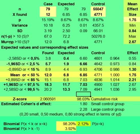 When
we do not study the whole population, but base our judgement on a
sample of the population, a critic could ask: So what? This
could be just a snapshot, not the big picture in space and time.
Determining the statistical significance is needed to evaluate the
reliability of the found effect size. This is done by calculating
confidence interval (ci) involved.
When
we do not study the whole population, but base our judgement on a
sample of the population, a critic could ask: So what? This
could be just a snapshot, not the big picture in space and time.
Determining the statistical significance is needed to evaluate the
reliability of the found effect size. This is done by calculating
confidence interval (ci) involved.
In this case Sun in Taurus (12 found, 6,85 expected, effect size is 1,75) was found 75% more often than expected. Sun in Taurus was found 6 times more often than Sun in Aquarius (2). Nevertheless, a large part of the found differences could be found by chance, given the small sample size of 79.
To understand in practice the statistical rules involved with it, we can look at the Expected values and corresponding effect sizes using the spreadsheet presented before. This time we fill in found values in the case (12 out of 79) and control groups (4771 out of 55047) in the yellow area (picture on the left). What do we see?
According to the large control group the expected value for Sun in Taurus is 6,85 (having the small 95% confidence interval of 6,66 - 7,03 based on a large control group). We found 12 in a sample of 79. With that small sample size the sampling error will blur the result and values between 1,9 (2) and 11,7 (12) could be expected in 95% of randomly selected ADB samples (third lower column). So getting 12 out of 79, would only hint to a borderline positive effect. This is also indicated by binomial risk values of 3,92 % (last value), which would not be significant in a 2-sided test with an alpha of 0,05.
We see that for Sun in Taurus the found value 12 against 6,85 expected, has an estimated effect size of 1,75. But if we take into account an error range of +/- 1,96 standard deviations (using an alpha of 0,05) because of the sampling error, the found value of 12 could hint to sub-population risks from 5,7/79 to 18,3/79. The corresponding effect sizes range from 0,84 to 2,67. So there could be a small negative correlation as well.
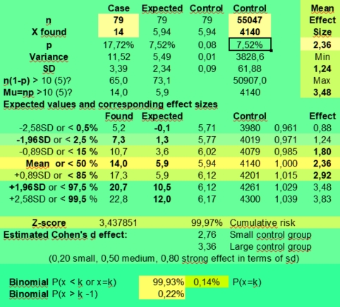 We
also found 14 times Jupiter in Gemini under art critics,
against 6 (5,94) expected. In this case we have a strong positive
association between Jupiter in gemini and art critics with an effect
size of 2,36 (1,24 - 3,48). We would have calculated an effect size
of 2,13 (1,12 - 3,14) when using +55047/12 as the expected value.
We
also found 14 times Jupiter in Gemini under art critics,
against 6 (5,94) expected. In this case we have a strong positive
association between Jupiter in gemini and art critics with an effect
size of 2,36 (1,24 - 3,48). We would have calculated an effect size
of 2,13 (1,12 - 3,14) when using +55047/12 as the expected value.
The found value of 14 clearly lies outside the range of expected values for Jupiter in Gemini (1,3 - 10,5) from a random ADB sample found in 95% of the cases. For this reason the difference would be called statistical significant.
The probability of getting a value of k > 13 in the binomial distribution with p is + 4140/55047 and n is 79 is only 0,22%. It would be 0,54% if we would have used p is 1/12. Both values are significant at an alfa level of 0,05. The value based on the actual probability of getting Jupiter in Gemini from an ADB sample is also significant at an alpha level of 0,01, having an expected range 0- 12,0.
So the NULL hypothesis could be rejected, which implies that not the expected values in the third row, but the found values in the second row would give the best estimate of having Jupiter in gemini for an art critic.
The found value of 14 also has 95% confidence interval. It the lies between 7,3 and 20,7. The Min and Max values (1,24 - 3,48) of the estimated effect size (2,36) are based on them. And in 70% of sampling cases effect size would be between 1,80 and 2,92.
But when using the 0,01 alpha criterion to estimate the effect size, because we got this result via selectively looking for special cases in large tables (data mining), there could still be a small negative effect size as well. As the found value of 15 has a 99% confidence interval of 5,2 to 22,8 corresponding to an effect size between 0,88 and 3,84 expected in 99% of cases. Taking this into account, getting 14 cases out of 79 would not be an extremely unexpected hit, unless astrologers before us would have observed and published similar data using another database having different members. Then we could accept a smaller alpha, or maybe a one-sided test. But this requirement might become problematic, because as far as we know, most astrologers doing research use the ADB as their reference point. And of course one cannot test any astrological hypothesis based on ADB categories by studying the same or slightly modified data again. And there is certainly no reason to test the usual vague could and might be statements found in astrology books that will fit any theory or finding and thus are not predictive at all.
In this article the focus is on the application of basic statistical tools to evaluate astrological data. We do not delve into unnecessarily statistical details, but try to explain modern statistical concepts by providing simple examples using real cases and what if scenario's. Our purpose is that astrology students try these tools for themselves, learning from a large astrological database that also provides reasonable control groups, instead of relying on the classic astrological dogma's, that were refuted so many times.
The try astrology for yourself and see if it works method is fallacious. It leads to similar problems as the statement: Migrants are criminal, just study the news and see what I mean. But using statistical techniques to evaluate ADB categories, just to check certain astrological assumptions, is another thing. And if you do it in a sophisticated way, like a criminologist studying the crime rates of migrants, you would also check for confounding factors like legal status, income, sex, age, race and education, just to name a few factors that are known affect crime rates. The last study would need complex multivariate analysis.
But our calculations are rather simple, as we did not deal with many other factors than those found in the control group. So let us show them for Venus in 9th house, where we found 13 cases out of 79 (probability = 13/79 = 16,5 %), against 79 times 1/12 (8,3%) is 6,58 expected. Because the risks involved with Placidus houses are not exactly 1/12, we used the actual found values for Venus in 9th house in the ADB control group. The calculated risk is 4463 cases found divided by the sample size 55047 is 8,11 % and 79 times that risk gives 6,41 cases expected (np). The effect size would then be the found risk of 16,5% divided by expected risk 8,11 % is 2,03. If we would have used 1/12 as the expected risk, the effect size would have been 1,97. So far we calculated risks as most astrologers would do.
Astrologers would then study Google or their astrology books for Venus in the 9th house and look for a fitting text like: This placement shows that pleasure is derived from study of philosophy, religion, and art. Their argument could then be: We found in the ADB twice as much Venus in 9 under art critics. Venus is associated with pleasure, art and money. The 9th house with the study of philosophy, religion and art. Art critics deal with all of them. So we do have a case for astrology.
The above argument looks sound. It is certainly better than the vague speculations found in astrology books, as its first premise “We found in the ADB twice as much Venus in 9 under art critics” is specific and can be checked. The symbolic associations might also be fitting, but the problem with them is that they tend to be too general to be predictive. What about the other planets? What about the whole picture? Which values do fit astrological expectations and which do not? Where do we deal with the sampling error or some other form or bias, and where not?
|
H1 |
H2 |
H3 |
H4 |
H5 |
H6 |
H7 |
H8 |
H9 |
H10 |
H11 |
H12 |
Total |
|
|
Sun |
4 |
6 |
7 |
6 |
5 |
7 |
7 |
6 |
6 |
11 |
7 |
7 |
79 |
|
Moon |
10 |
8 |
8 |
6 |
4 |
10 |
5 |
7 |
10 |
2 |
5 |
4 |
79 |
|
Mercury |
5 |
4 |
6 |
7 |
7 |
7 |
4 |
9 |
8 |
10 |
5 |
7 |
79 |
|
Venus |
7 |
9 |
8 |
3 |
6 |
5 |
5 |
9 |
13 |
4 |
5 |
5 |
79 |
|
Mars |
6 |
6 |
3 |
2 |
7 |
7 |
11 |
12 |
6 |
5 |
10 |
4 |
79 |
|
Jupiter |
4 |
7 |
5 |
11 |
10 |
8 |
8 |
9 |
6 |
4 |
4 |
3 |
79 |
|
Saturn |
8 |
6 |
6 |
11 |
2 |
8 |
8 |
5 |
7 |
9 |
3 |
6 |
79 |
|
Uranus |
6 |
4 |
7 |
4 |
4 |
7 |
13 |
5 |
8 |
9 |
6 |
6 |
79 |
|
Neptune |
3 |
6 |
5 |
11 |
11 |
7 |
4 |
5 |
5 |
6 |
9 |
7 |
79 |
|
Pluto |
4 |
5 |
9 |
6 |
11 |
6 |
7 |
3 |
8 |
8 |
7 |
5 |
79 |
|
N Node |
6 |
10 |
2 |
6 |
5 |
6 |
5 |
7 |
12 |
6 |
7 |
7 |
79 |
|
Chiron |
9 |
6 |
9 |
5 |
3 |
4 |
11 |
10 |
3 |
7 |
6 |
6 |
79 |
Finding clear group patterns of planet in house of ADB categories that reflected the symbolic meaning of the astrological houses would provide a strong case for astrology, but the not that striking patterns as found under art critics and plumbers can also be found in random ADB samples. Any found variation around an expected mean due to the sampling error could of course be interpreted astrologically, but it would be something like attributing meaning to particular specks in a Rorschach inkblot test, when there is nothing special in it.
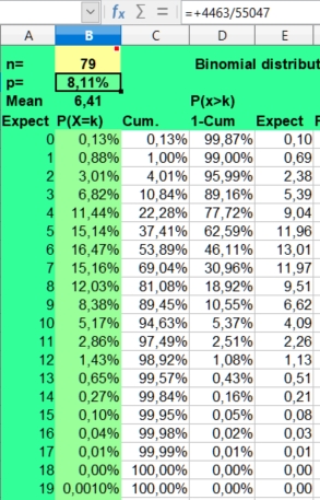 The
major problem with astrological research is that fluctuations around
the mean will always happen because of statistical variation. So, the
encountered 13 out of 79 cases of Venus in 9 against 6,41 cases
expected, could be the result of the Sampling
error, like the special case we described in Jupiter
in Gemini above.
The
major problem with astrological research is that fluctuations around
the mean will always happen because of statistical variation. So, the
encountered 13 out of 79 cases of Venus in 9 against 6,41 cases
expected, could be the result of the Sampling
error, like the special case we described in Jupiter
in Gemini above.
For this reason we must answer the important question: What effect size is large enough to be convincing?
In any ADB sample - being it a specific category or a random sample - most frequencies for Venus in 9 (13 found) would deviate around the expected mean of 6,41. Values between 4 (11%) and 8 (12 %) would be expected most of the times (81 minus 22 = 59%) according to the binomial distribution. But because they had little impact, a small effect size and little predictive value, empirically oriented astrologers would not pay much attention to them.
But what would for scientists and statisticians be an impressive effect size? Large deviations from the expected mean of course. What is large enough? Those values that distinguish group members from other groups, like the neck size of a giraffe or the impressive nose size of an elephant. If you knew that the neck size of an animal was very large, you could deduce that it could be a giraffe. The same with the nose of an elephant. You did not need statisticians to see the differences between species.
But when group differences become smaller, there will be overlap between case and control groups, and statistical methods are needed to describe them with more precision than vague terms as “could be” or “might be” can do. A smoker could get lung cancer. A not smoker can have lung cancer as well. Both are true statements, but they are not predictive. You cannot base decisions on them. You need the actual risks involved with those events with an estimate of their confidence intervals. But to statically proof that smoking causes lung cancer, now an established fact, epidemiologists had to compare and follow-up large case and control groups for many years, as well as decipher the underlying biochemical causal mechanisms by other means.
To empirically find out if a found astrological value in a ADB category with a certain sample size n is statistically seen different from the ADB as a whole, we have to count its astrological properties and compare them to as many as possible similar samples that were randomly taken from the ADB. Having a quick glance at the ADB and just relying on your astrological experience would not deal with the sampling error. On the contrary: Your by prior experience biased method would become part of the problem instead of solving it. For this reason you need to do assumptionless research to get rid of the selection bias of your expectations. An objective researcher of truth should have no preferences that might favor one outcome above the other.
To get enough control samples to see statistically significant differences with a confidence interval of 95%, one should actually create and study thousands of random samples of 79 members from the ADB, to see if and how often individual counts differed from the found values in the study group. If only 2% of the random control samples had similar values with regard to Venus in 9 in our study group, then the conclusion could be drawn that in our selected sample of art critics, Venus in 9 happened significantly more often than found in thousands of random ADB samples. As the 2% cases found in random samples, would be smaller than the 2,5 % of lowest and 2,5 % of highest values a two sided test with a 95 % confidence interval.
But doing such an laborious sampling experiment is not needed, since the rules involved with random sampling have been meticulously studied by statisticians. They provided us formulations and curves like the normal distribution which can be used to predict the outcomes of most sampling experiments. And because the statistical properties of the ADB and its sub-categories have been studied in detail by the ADB Research group, doing statistical research on the ADB categories has become a piece of cake. But accepting its outcomes might be more difficult problem to digest.
The major question is then, does this sample of 79 art critics contain unexpectedly high or low values that would also quite often show up in randomly selected ADB samples? If the answer is: Yes, this value would happen in more than 1 in 20 random ADB samples with this sample size, the NULL hypothesis would be accepted, which implies that the differences found in this sample were not large enough to be statistical significant with an alpha 0,05. They could have just been by chance findings. They would just by chance happen in 1 of the 20 random samples with n is 79 found in the ADB. Could you predict with it with a reasonable amount of confidence? Probably not.
But if one or more found values (say: Venus in 9 under art critics) did not pop up that regularly in many random ADB samples (say less than once in 20 random ADB samples with an alpha of 0,05 or less than once in 100 with an alpha of 0,01) , the found value would be called significant. Then the NULL hypothesis would be rejected and the found values would be accepted as typical for the study group, and not just be regarded as a likely product of statistical variation and chance.
The found and expected values are found in the upper rows: N(umber) referring to sample size in case and control groups (yellow), X found to actual found values in case and control groups (yellow). But you see here also what is to expected in the Case (n=79) and Control (n=55047) and thus Expected groups (Based on n=55047, thus having a much smaller confidence interval than just a sample of 79 cases) .
We used a simple formula to estimate variance and the standard deviation SD: Var = SD^2 = np(1-p). It can be applied when n(1-p) and np are larger than 5 (or better 10). Much more details can be found on Wikipedia pages of the Normal distribution and the Binomial distribution.
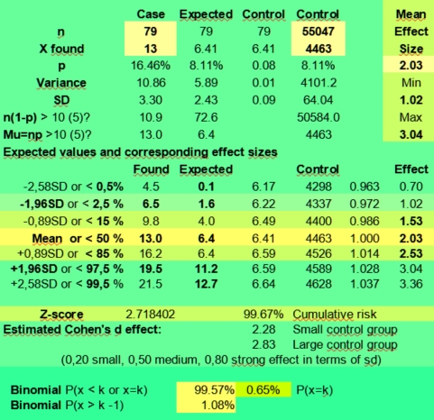 When
the standard deviation is known, confidence intervals of
expected values (based on large or small control groups) and found
values can be easily calculated. They are found under Expected
values and corresponding effect sizes in the green calculator
in the lower rows.
When
the standard deviation is known, confidence intervals of
expected values (based on large or small control groups) and found
values can be easily calculated. They are found under Expected
values and corresponding effect sizes in the green calculator
in the lower rows.
The 95 % confidence interval is given by np + /- 1,96 times the SD. For the expected values derived from the large control group it is 6,41 + /- 1,96 times 2,43, having a range of 1,6 to 11,2.
The found value of 13 falls outside that range of in 95% of cases expected values. So the Null hypothesis would be rejected. The effect size would be between 1,02 and 3,04.
The 99 % confidence interval is given by np + /- 2,58 times the SD. It is thus 6,41 + /- 2,58 times 2,43, having a range of 0,1 to 12,7. The found value of 13 would fall just outside that range, so the Null hypothesis would also be rejected. The effect size would be between 0,70 and 3,36.
But according to the binomial distribution values > 11 have a risk 0 2,51 % , values > 12 would have a risk of 1.08 %. The value of 13 would thus not be significant using the 99% confidence interval.
Cohen's d value of 2,83 (for a large control group) for Venus in 9 was predicted using the estimated variance values. The estimated SD for Venus in sign in the control group (64,04) was much smaller than actual found (420). The actual found Cohen's d value was 3,27, which is 30% away from the formula predicted. The effect size value of Cohen's D is explained in a later chapter.
We could look for other values that fall outside the in 95% of cases expected values of a random ADB sample of 79. In a contingency table of 144 values, say for 12 planets in sign or house on average 7,2 (c.i. 3-13) of them could be expected. See: Data mining. When using a 99% confidence interval the expected false positive value would still be 1,44 (0-4). So finding some some of them in a table of 144 items would not yield a case for astrology. This would be the expected false positive type 1 error dealing with random samples. Our finding for Jupiter in Gemini is likely to be one of them as we (1) deliberately cherry-picked that interesting us high value out of a table with 144 items and (2) that value was not really an outlier far away from the expected mean. When we encountered meaningful patterns of outliers - values far away from the mean - that were also fitting astrological theories, that would not be business as usual. Finding astrological patterns in the data is important, as probability calculations can predict how often exceptionally high or low values will occur once in the many samples (say 1 in 20 with an alpha of 0,05), but not when and where they would exactly be found.
So if political leaders as heads of state were predicted to have more likely a Leo Sun, Moon or Ascendant, getting high values on those positions could confirm an astrological theory. And if they were not found in large ADB samples, that theory should be rejected. Astrologers assume that other astrologers did this kind of research before. But astrology books never provide quantitative data to proof their point. So the astrology cookbooks have to be rewritten.
Effect size can be compared to Relative Risk (RR) or risk ratio's. But we cannot equal our effect size with relative risk. Nevertheless, the effect size values for small categories would not differ that much from relative risks because of the large control group.
Relative Risks deal with the effect of some to be controlled independent variable (exposure to some pathogen) on the occurrence of the to be measured later dependent variable (a particular disease). The relative risk would then be the amount of disease cases after exposure to the pathogen divided by amount of disease cases without prior exposure to the pathogen during a particular follow-up period.
For practical reasons we did not compare the astrological properties of the category art critics with all the ADB entries minus the 79 art critics. We compared the astrological properties of the different categories to all timed ADB entries of persons for two reasons. First because it takes two weeks to calculate such a large control group and second because we wanted to use the same control group for all categories. Using the same ADB control group for all categories enabled us to compare the different effect sizes and other statistical values found in the different categories. As they were calculated from the same source in the same way, the relation between case and control groups will always be clear.
The above details sound rather abstract and technical, so we now present a simple astrological question to show the statistical details. Because all the calculations are done using one spreadsheet and only four values need to be known, the example demonstrates that it is not that difficult to estimate confidence intervals today. Entering birth data in an astrology program takes more time.
The provided values used are just imaginative, as no astrologer, including C.E.O Carter, ever studied accidents seriously using modern standards. But I appreciate his book The astrology of accidents , because Charles Carter tried to be objective. He provided astrological facts as they were, instead of focussing on popular astrological opinions. But Carter did not use control groups. And the predictive value of his study is low. How could his study be done again? Just a thought experiment.
The relative risk of getting a major accident during a Mars conjunct Ascendant transit would be the proportion of people having an accident during the transit (say 5% or 5 accidents per 100 affected people) divided by the proportion of people having such an accident in a comparative time-span without having that particular transit (say 2% or 20 accidents per 1000 people). The relative risk would then be 2,5 with a 95% confidence interval of 0,34 to 4,64 using a normal distribution approach (see the picture below on the right). This corresponds to expected values between 0 and 4,7 (5) in 95% of samples with n is 100 (third row).
![]()
The
large confidence interval of the effect size 0,36 to 4,64 implies
that there still could be no astrological effect at all. This was the
major problem in Charles Carter classic study of 168 accidents.
A similar problem is that the 20 out of 1000 cases found in the control group can not provide a reliable estimate of the mean. The 95% confidence interval of this estimate is 11,3 - 28,7 (5th column), so the expected risk of 2,0 % has also a wide 95% confidence interval of 1,1 - 2,9%. The more exact approach using the binomial distribution with p=0,02 and n is 1000 (picture below) shows that 12 to 29 are the most expected values, corresponding to an estimated risk of 1,2 - 2,9 % of having an accident without having a Mars conjunct ascendant transit.
But when 100.000 people would have 2000 accidents in a certain time-span, the estimated risk of 2,0 % would have a confidence interval of 1,91 - 2,09 %. There is only one problem: Rates on accidents as above could be retrieved from official instances or insurance companies, but not with the guarantee that the victims did not have a Mars conjunct ascendant transit at that time! So you had to do this study yourself, including the calculating of more than 100.000 ascendants, to meet this criterion.
The good news is that the Null hypothesis expects that the risk of having an accident would be the same with or without that transit. The small proportion in the control group that would have a Mars conjunct ascendant transit could be estimated based on theoretically or empirically expected values as in The actual risks involved with aspects. Their small impact on the control group could be estimated from the increased risk in the case group, when the Null hypothesis was rejected. So it would not be necessary to retrieve the birth certificates of 100.000 + 100 people to calculate their Ascendant, calculating 100 of them in the case group would suffice. But getting 5 accidents out of 100 against 2 (+/- 0,09) expected would not yield a positive predictive effect size with a confidence interval of 0,36 to 4,64. So the Null hypothesis had to be accepted (type 2 error).
But if more observations in the study group were done and 50 accidents per 1000 affected people could be recorded, then the same relative risk of 2,5 would be much more convincing with a confidence interval of 1,81 - 3,18. See the picture below. In this case 1000 ascendants had to be calculated.
The two tables above and below allow us to compare different methods with different sample sizes. We first used the normal distribution, but because of the small np = 5 (> 10 preferred) and we deal with discrete numbers, applying the discrete binomial distribution is a much better approach.
According to the binomial table above, the risk of getting K is 5 out of 100 with p = 20/1000 is 3,53%. The risk of getting 5 or more is 5,08%, so this is still a borderline case, as only getting 6 or more cases (p = 1,55%) would be statistical significant at the 0,05 level. So, we did not have a case for astrology.
But getting 50 accidents out of 1000 affected natives, would be extremely significant, as the most expected values around the mean would be 12 to 28. Significant values would be k < 11 (p = 2,04%) and k > 29 (p = 2,07%), 11 and 29 being borderline values. As you can see the rough estimate using the normal distribution gives a similar range of 11,3 - 28,7 expected (third column on the right).
The risk of getting 50 accidents out of 1000 cases when 20 were expected is 4,92 E-9 and the risk of getting 50 or more would be 7,88 E-9 or 0,00000000788. But you could not claim this doing only some observations. Here astrology books can easily misguide you, as their writers never used control groups. They just assumed things. But a Santa Claus story that is repeated many times in a tradition, still remains a story.
![]()
According
to the continuous Poisson sampling distribution the risk of 5
out of 100 cases when 2 were expected is 3,61% (or 5,27% for 5 or
more). Again we have a borderline positive effect, as as only getting
a value of 6 or higher (p = 1,66) would be statistical significant at
the 0,05 level.
And again, getting 50 accidents out of 1000 affected natives when 20 were expected, would be an extremely significant result, as values from 12 (Px <12 is 3,90%) to 29 (Px > 28 =3,43%) could be expected in 95% of the cases. The Poisson distribution estimates the risk of getting 50 out of 1000 when 20 were expected as 7,63 E-9 and the risk of getting 50 or more would as 1,25 E-8 or 0,0000000125.
With those numbers astrologers really had a case. But how often astrologers study aspects in the quantitative way? And if they found a reliable effect size of 2-3, would it be predictive? Well, only in high risk situations or when labile and suggestible people panic because of bad fortune telling.
But after consulting an astrologer, you could get a little bit nervous. So, the small increased accident proneness could become a self fulfilling prophecy of which the sociologist William Isaac Thomas said: If men define situations as real, they are real in their consequences. Then both a small real effect and a potential strong imaginative effect would combine to increase the risk.
But realise that, how impressive this fictive case for astrology might appear, 95% of the people having that transit would not have an accident!
To study the significance of differences found in the rows of observed and expected values, the chi-square value of the 12x2 tables were calculated.
The chi-square value is the sum of the squares of the difference between the twelve (n) pairs of found (O) and expected (E) frequencies of planet in sign divided by the expected values, which is shown as the last value under Total in the table below.
In formula: X^2 = S (O-E)2 / E, where the symbol sigma (S) denotes the sum.
|
Aries |
Taurus |
Gemini |
Cancer |
Leo |
Virgo |
Libra |
Scorpio |
Sag |
Cap |
Aqua |
Pisces |
Total |
|
|---|---|---|---|---|---|---|---|---|---|---|---|---|---|
|
Sun in sign observed (O) |
9,00 |
12,00 |
8,00 |
10,00 |
9,00 |
5,00 |
4,00 |
5,00 |
3,00 |
5,00 |
2,00 |
7,00 |
79,00 |
|
Sun in sign expected (E) |
6,80 |
6,85 |
6,85 |
6,75 |
6,79 |
6,47 |
6,49 |
6,11 |
6,02 |
6,38 |
6,60 |
6,88 |
79,00 |
|
O-E |
2,20 |
5,15 |
1,15 |
3,25 |
2,21 |
-1,47 |
-2,49 |
-1,11 |
-3,02 |
-1,38 |
-4,60 |
0,12 |
0,00 |
|
(O-E)2 |
4,84 |
26,55 |
1,33 |
10,58 |
4,89 |
2,17 |
6,20 |
1,24 |
9,11 |
1,92 |
21,19 |
0,01 |
89,92 |
|
(O-E)2 / E |
0,71 |
3,88 |
0,19 |
1,57 |
0,72 |
0,34 |
0,96 |
0,20 |
1,51 |
0,30 |
3,21 |
0,00 |
13,59 |
For Sun in Aries the (O-E)2 / E value is calculated as (9 - 6,8)^2 / 6,8 = 0,71. This is repeated for the other sun signs in the above rows. Of course the sum (Total) of all the observed minus expected values should always be zero, but the S (O-E)2 values of rows are seldom zero. Because of the sampling error the most likely outcomes having S (O-E)2= 0 are seldom found. And that empirical fact goes against human intuition.
For Sun in sign in the group Art critic the S (O-E)2 is 89,92. The X^2 value is the sum of (O-E)2 / E which is 13,59. What does that imply?
From the X^2 values of rows like planet in sign or house, we can calculate the risk that the found values were caused by the sampling error. We use those risks in a statistical test, the chi-squared test for categorical data , to find out how much the found frequencies of specific ADB categories do differ from random samples of the ADB. When calculating confidence intervals of found values with the help of the binomial and normal distribution we did the same. But because of the small numbers involved in this study group, it was very difficult to show any statistical significant effect. But when comparing twelve pairs of found and expected frequencies at once, instead of many individual pairs, the test becomes much more sensitive.
The X^2 values are relative and not absolute measures of the found differences, as the observed minus the expected frequencies are divided by the expected frequencies. This results in a kind of normalisation enabling comparisons to be made between similar X^2 tables. And just as in the related concept of variance, proportionally large differences between found and expected frequencies are stressed, because their differences are squared. So when a planet in sign or house does matter for a certain ADB category, it should result in outliers in the tables, leading to much more variance than could be expected by chance alone.
Similar X^2 tables will have the same degrees of freedom. The larger the amount of cells to be compared, the larger the possibility that there will be differences, the larger will be the degrees of freedom. But if we would define found x is is a function of y expected, we had zero degrees of freedom. In this case a plot could be drawn that would show you a straight line, circle, ellipse or any other linear point-to-point relation depending on the mathematical formula. But that regularity is more typical of astronomical rules than of astrological rules, because astrological rules typically deal with stochastic events with a particular risk.
The general formula for the degrees of freedom when comparing tables of found and expected values is: Degrees of freedom = (amount of columns minus 1) multiplied by (amount of rows minus 1). The underlying idea of is that when you know the values of the row or column totals, any other value is determined by the totals minus the frequencies of the known other values in the row or column. For typical astrological evaluations with 12x2 tables of observed against expected frequencies the degrees of freedom are (12-1) * (2-1) = 11 degrees of freedom.
Low X^2 values indicate situations where the found values are close to the expected values in random samples from the population. Statistically seen nothing special happened for that row, as similar findings could be reproduced when doing the experiment again with randomly selected ADB samples.
When comparing small groups of ADB categories or individual clients with an expected value per record of np is 5 or lower (60 or less cases), the statistical noise is substantial. Large differences could just be caused by chance (sampling error), so there will be a large grey area where relevant effect sizes could occur that will not reach enough statistical significance to be accepted as “real effects” by statisticians (type II error). Astrologers might feel that this type II error can at times be very crude, when they encounter in small scale astrological research impressive results that are not yet statistically significant. But statisticians would invite them to find in an objective way just some more randomly found cases to prove their point. As you cannot proof that a dice is false after only a few throws. But repeating patterns found in the sky as well on earth could proof your empirical point.
Statisticians empirically found out that the X^2 values of frequency tables of found and expected values of a certain size (degrees of freedom) can be linked to probabilities. What is calculated is the risk that we deal with the sampling error, which is the error caused by observing a sample instead of the whole population. The smaller the sample, the greater the effect of the sampling error, and the greater the risk that your sample does not fully reflect the real population under study.
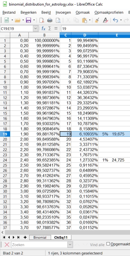 High
X^2 values hint to more significant differences
between the found and by chance expected frequencies. Then something
special might be happening here, being it an astrological effect or
not. For slow planets in sign Zeitgeist could play a major role, but
for slow planets in house and personal planets it would be
interesting to study the rows where unexpected variation does occur,
as this could hint to astrological factors being involved in a
particular (sub)category.
High
X^2 values hint to more significant differences
between the found and by chance expected frequencies. Then something
special might be happening here, being it an astrological effect or
not. For slow planets in sign Zeitgeist could play a major role, but
for slow planets in house and personal planets it would be
interesting to study the rows where unexpected variation does occur,
as this could hint to astrological factors being involved in a
particular (sub)category.
Which X^2 values hint to something special happening in a particular area? What is special? Something that is according to statisticians not business as usual. For astrologers many significant events they interpret might seem business as usual, but statisticians want to quantify this subjective qualification.
And there is good reason to do so according to mathematicians studying the problems of complexity like Pythogoras who stated that four is all: As 1+2+3+4=10/1. A new beginning after only four opinions. For
On the left you see tables of X ^2 values with 11 degrees of freedom C linked probability D that the found differences between the two rows could be due to chance.
The for astrology most important X^2 value is 19,675 for a 2-sided test with an alfa of 0,05. Values higher than this would be called statistically significant at the 5% significance level. The other significant value is 24,725 for a 2-sided test with an alfa of 0,01 (1% significance level).
When studying very large samples, tiny differences might statistically seen be very significant. But in this presented case an effect size of 2 between found and expected values would suffice according to the standard 5% criterion.
Notice that squared values are always positive, so high X^2 value can both refer to positive (RR > 1) or negative (RR<1) correlation coefficients. A two sided test is needed when the actual population frequencies are not known. This is the case for most astrological questions, even though astrology books suggest otherwise.
Questions like: Which house or planet rules art critics could be answered by observing high (preferably > 19,678) X ^2 values in the X ^2 row of that planet or house. They would statistically been seen the best guess. Traditional suggestions based on astrological symbolism are obsolete. In our study of art critics the 2-8 axis seemed to be most relevant. And of the personal planets in sign Jupiter and Mercury score the best.
But the interpretation of findings in rows with low X^2 scores makes little sense, as the found differences are most likely the product of chance or irrelevant side-effects. The results resemble the expected random results of throwing a 12-sided dice. The next time you would repeat the experiment with other members of that same category, you would probably see quite another pattern.
The statistical test we then use is the chi-squared test for categorical data , where the found and expected frequencies are determined by the distribution and categorisation of the ADB. The research question could be stated as: When we selectively pick out entries the sub-category Vocation Art Critic from the ADB, do we get a sample that really differs from a random sample of the ADB? In case astrological factors do not matter for that category, which we call the NULL hypothesis, the distribution of frequencies found would resemble a random sample from the ADB. But if we find a X ^2 value above 19,675 for a 2-sided test, which is only found in 5% of the cases just by chance, the NULL hypothesis could be rejected. Then we have to consider the alternative hypothesis, which states that astrological or other factors do play some role.
An astrologer might complain that astrological factors still could matter even the results of test were disappointing. That is correct. The on paper best football team can at timer have disappointing results. Then more matches should be observed. But it would be unprofessional to blame the arbiter for the lost match.
|
Aries |
Taurus |
Gemini |
Cancer |
Leo |
Virgo |
Libra |
Scorpio |
Sag |
Cap |
Aqua |
Pisces |
Total |
P% |
|
|---|---|---|---|---|---|---|---|---|---|---|---|---|---|---|
|
Sun |
0,71 |
3,88 |
0,19 |
1,57 |
0,72 |
0,34 |
0,96 |
0,20 |
1,51 |
0,30 |
3,21 |
0,00 |
13,59 |
25,7 |
|
Moon |
0,07 |
0,97 |
0,42 |
0,92 |
0,85 |
0,36 |
0,34 |
3,16 |
0,03 |
0,28 |
0,81 |
1,07 |
9,29 |
59,5 |
|
Mercury |
1,10 |
0,54 |
4,12 |
0,00 |
2,13 |
1,01 |
2,10 |
0,00 |
1,24 |
2,23 |
0,60 |
0,62 |
15,69 |
15,3 |
|
Venus |
0,13 |
0,66 |
0,03 |
2,91 |
1,64 |
0,31 |
0,44 |
1,01 |
0,29 |
0,45 |
0,26 |
0,27 |
8,41 |
67,6 |
|
Mars |
3,21 |
0,01 |
1,28 |
0,37 |
1,92 |
1,24 |
0,81 |
0,18 |
0,01 |
1,01 |
1,08 |
0,03 |
11,13 |
43,2 |
|
Jupiter |
0,19 |
0,62 |
10,93 |
1,96 |
0,19 |
0,02 |
0,84 |
0,02 |
0,16 |
1,79 |
0,00 |
1,51 |
18,23 |
7,6 |
|
Saturn |
0,20 |
1,43 |
0,59 |
1,36 |
0,03 |
0,21 |
0,13 |
0,16 |
0,76 |
0,45 |
1,23 |
0,09 |
6,64 |
82.7 |
|
Uranus |
0,33 |
0,53 |
0,09 |
0,25 |
0,01 |
0,00 |
1,41 |
0,57 |
2,29 |
1,54 |
0,29 |
0,04 |
7,36 |
76,9 |
|
Neptune |
7,08 |
5,43 |
0,64 |
4,21 |
0,22 |
0,41 |
4,08 |
4,30 |
1,84 |
0,19 |
2,15 |
4,29 |
34,82 |
0,0 |
|
Pluto |
0,17 |
28,59 |
1,97 |
0,19 |
3,18 |
5,38 |
2,92 |
0,23 |
1,12 |
0,66 |
0,53 |
0,07 |
45,01 |
0,0 |
|
N Node |
0,71 |
2,77 |
1,32 |
1,24 |
0,06 |
1,04 |
0,38 |
1,19 |
0,77 |
0,01 |
0,32 |
4,32 |
14,13 |
22,6 |
|
Chiron |
0,03 |
1,64 |
3,33 |
0,02 |
0,43 |
0,18 |
1,31 |
2,02 |
2,42 |
0,43 |
0,63 |
0,39 |
12,84 |
30,4 |
In this case rows of Sun (25,7%), Mercury (15,3%), Jupiter (7,6%), the North node (22,6%) and other planets in sign, have X^2 values that clearly exceed the 50-50, just throw a penny, neutral position. But they are not significant using the 5% criterion. So you could not reliably predict or explain facts with it.
Jupiter in gemini (effect size 2,36, range 1,21 - 3,50) contributes most to the relative high X^2 score of its row. Even a beginning astrologer could without doubt explain this. But it could also be an outlier, that would not be repeated with another sample of art critics. Remember that this finding comes from a 12 times 12 contingency table in which we could expect 144/20 is 7,2 cases to be unexpectedly high or low just by chance using an alpha of 0,05. This results in the type 1 error, assigning significance to an outcome, when there is nothing special happening (false positive).
The X ^2 values for Neptune and Pluto are very significant, but here the problem is that we did not match the control group for birth year. Astrological factors could play a role, but here we primarily deal with Zeitgeist as a relevant background to keep into consideration, as the ADB is not equally distributed in time. The profession of art critic is also likely to be unevenly distributed in time and place. So, sociological and cultural historical factors could be better in predicting the outcomes of the slow planets times than mundane astrologers could do. But if they found relevant repeating patterns in time according to slow planets, they could have a point.
The Placidus house cusp positions yielded significant results on the 2-8 axis ( X^2= 21,4, p is 0,029 with 11 df).
|
Aries |
Taurus |
Gemini |
Cancer |
Leo |
Virgo |
Libra |
Scorpio |
Sag |
Cap |
Aqua |
Pisces |
Total |
P(%) |
|
|---|---|---|---|---|---|---|---|---|---|---|---|---|---|---|
|
Cusp 1 |
0,03 |
0,04 |
0,08 |
1,97 |
0,01 |
0,02 |
3,68 |
0,31 |
0,00 |
3,98 |
0,03 |
0,03 |
10,18 |
51,4 |
|
Cusp 2 |
1,29 |
0,29 |
0,95 |
0,40 |
1,10 |
0,01 |
0,17 |
4,54 |
0,90 |
1,90 |
9,81 |
0,05 |
21,40 |
2,9 |
|
Cusp 3 |
1,46 |
0,20 |
0,69 |
0,03 |
1,42 |
0,16 |
0,10 |
0,05 |
2,67 |
0,30 |
1,37 |
4,48 |
12,92 |
29,9 |
|
Cusp 4 |
0,68 |
2,01 |
0,44 |
0,11 |
0,06 |
0,68 |
0,02 |
0,03 |
0,09 |
1,38 |
0,34 |
0,17 |
6,00 |
87,3 |
|
Cusp 5 |
0,48 |
2,14 |
0,93 |
0,07 |
1,56 |
0,04 |
0,34 |
1,42 |
0,19 |
0,02 |
0,75 |
0,11 |
8,03 |
71,1 |
|
Cusp 6 |
0,05 |
1,04 |
7,80 |
1,78 |
1,88 |
0,41 |
0,46 |
0,95 |
0,98 |
0,01 |
0,00 |
1,04 |
16,41 |
12,7 |
|
Cusp 7 |
3,68 |
0,31 |
0,00 |
3,98 |
0,03 |
0,03 |
0,03 |
0,04 |
0,08 |
1,97 |
0,01 |
0,02 |
10,18 |
51,4 |
|
Cusp 8 |
0,17 |
4,54 |
0,90 |
1,90 |
9,81 |
0,05 |
1,29 |
0,29 |
0,95 |
0,40 |
1,10 |
0,01 |
21,40 |
2,9 |
|
Cusp 9 |
0,10 |
0,05 |
2,67 |
0,30 |
1,37 |
4,48 |
1,46 |
0,20 |
0,69 |
0,03 |
1,42 |
0,16 |
12,92 |
29,9 |
|
Cusp 10 |
0,02 |
0,03 |
0,09 |
1,38 |
0,34 |
0,17 |
0,68 |
2,01 |
0,44 |
0,11 |
0,06 |
0,68 |
6,00 |
87,3 |
|
Cusp 11 |
0,34 |
1,42 |
0,19 |
0,02 |
0,75 |
0,11 |
0,48 |
2,14 |
0,93 |
0,07 |
1,56 |
0,04 |
8,03 |
71,1 |
|
Cusp 12 |
0,46 |
0,95 |
0,98 |
0,01 |
0,00 |
1,04 |
0,05 |
1,04 |
7,80 |
1,78 |
1,88 |
0,41 |
16,41 |
12,7 |
In the case of art critics in the ADB finding significance at the 2-8 house axis symbolically seems to make sense. As the second house of Venus and Taurus is associated with creating and attributing value and the opposite 8th house of Mars, Pluto and Scorpio is associated with probing attributed value.
If you look at the effect sizes involved, you see that Cusp 2 in Aquarius and Cusp 8 in Leo are found 2,4 times more often than expected and that Cusp 2 in Scorpio and Cusp 8 in Taurus score 4 times less than expected.
|
Aries |
Taurus |
Gemini |
Cancer |
Leo |
Virgo |
Libra |
Scorpio |
Sag |
Cap |
Aqua |
Pisces |
Total |
|
|---|---|---|---|---|---|---|---|---|---|---|---|---|---|
|
Cusp 2 |
1,53 |
0,76 |
1,38 |
0,77 |
0,63 |
1,04 |
1,00 |
0,25 |
1,35 |
0,46 |
2,40 |
0,90 |
12,62 |
|
Cusp 8 |
1,00 |
0,25 |
1,35 |
0,46 |
2,40 |
0,90 |
1,53 |
0,76 |
1,38 |
0,77 |
0,63 |
1,04 |
12,62 |
Most astrologers do not interpret the slow planets in sign that much, but take into consideration their house positions. But the positions of the planets in Placidus houses were not significant at the 5% level.
|
H1 |
H2 |
H3 |
H4 |
H5 |
H6 |
H7 |
H8 |
H9 |
H10 |
H11 |
H12 |
Total |
P% |
|
|---|---|---|---|---|---|---|---|---|---|---|---|---|---|---|
|
Sun |
1,63 |
0,18 |
0,02 |
0,00 |
0,10 |
0,30 |
0,22 |
0,00 |
0,00 |
1,90 |
0,02 |
0,04 |
4,43 |
95,6 |
|
Moon |
1,86 |
0,33 |
0,28 |
0,05 |
0,98 |
1,84 |
0,44 |
0,05 |
1,81 |
3,18 |
0,42 |
1,10 |
12,32 |
34.0 |
|
Mercury |
0,80 |
1,47 |
0,12 |
0,08 |
0,21 |
0,26 |
0,57 |
1,87 |
0,41 |
1,47 |
0,69 |
0,03 |
7,97 |
71,6 |
|
Venus |
0,02 |
0,54 |
0,26 |
1,60 |
0,00 |
0,11 |
0,12 |
1,56 |
6,79 |
1,24 |
0,73 |
0,83 |
13,80 |
24,4 |
|
Mars |
0,09 |
0,08 |
1,88 |
2,89 |
0,07 |
0,14 |
3,32 |
4,52 |
0,04 |
0,53 |
1,40 |
1,33 |
16,31 |
13,0 |
|
Jupiter |
0,96 |
0,02 |
0,42 |
2,97 |
1,64 |
0,30 |
0,37 |
1,01 |
0,04 |
1,15 |
0,92 |
2,02 |
11,81 |
37,8 |
|
Saturn |
0,24 |
0,07 |
0,04 |
2,73 |
3,23 |
0,28 |
0,27 |
0,31 |
0,07 |
1,03 |
1,97 |
0,07 |
10,31 |
50,3 |
|
Uranus |
0,05 |
0,87 |
0,06 |
0,92 |
0,99 |
0,05 |
5,94 |
0,41 |
0,19 |
0,78 |
0,11 |
0,05 |
10,41 |
49,4 |
|
Neptune |
1,89 |
0,04 |
0,31 |
3,24 |
2,98 |
0,05 |
1,00 |
0,49 |
0,51 |
0,05 |
0,81 |
0,02 |
11,38 |
41,2 |
|
Pluto |
0,44 |
0,03 |
1,87 |
0,02 |
5,41 |
0,04 |
0,03 |
2,71 |
0,02 |
0,02 |
0,08 |
0,89 |
11,54 |
39,9 |
|
N Node |
0,04 |
1,89 |
3,08 |
0,04 |
0,46 |
0,06 |
0,35 |
0,04 |
4,16 |
0,06 |
0,02 |
0,01 |
10,20 |
51,3 |
|
Chiron |
0,95 |
0,04 |
1,05 |
0,37 |
2,03 |
0,99 |
2,87 |
1,87 |
2,02 |
0,01 |
0,05 |
0,07 |
12,32 |
34,0 |
The Mars differences between found and expected values could have been arisen in 13% of the cases just by chance. Because the X^2 values do not make a difference between strong negative and positive effects, it is good to compare them with Mars in the houses effect sizes presented before ().
Cohen's d value is a statistical effect size measure to indicate the differences between two groups. It is defined as the difference between two means divided by the pooled standard deviation of the compared groups. So it measures the differences between two means in terms of standard deviations.
Cohen's d = (MeanA - MeanB) / pooled standard deviation of A and B.
The pooled standard deviation (SD) is the square root of ((SDA2 + SDB2) / 2) or square root of ((VARA + VARB) / 2). It lies between the two SD values, being more close to the largest SD value of the compared groups. When using a large control group
When comparing ADB categories with the expected values of the ADB, we used for MeanA - MeanB the found value minus the expected value of each planet in sign or house. This according to the statistical rule that the found mean values, are the most likely estimates of the expected mean (np) we in this study have.
Variance was calculated by TkAstroDb as the actual found Sum of the squared differences of the mean divided by n-1 in the case and control group of expected values: VAR = S (O-E)2 / 11, the SD being the square root of it.
But for the binomial calculator the estimated value VAR = np(1-p) was used, as here only the found values and their sample sizes were used for input. The reduced data input results in inaccurate results, especially with small samples that are not normally distributed. It only gives a very rough estimated of Cohen's d effect size. Nevertheless, you could use this method to estimate effect sizes and confidence intervals, in comparisons where we cannot directly measure variance. Example of this method is given in The relative risk of having an accident during a Mars conjunct Ascendant transit and The calculation of the effectiveness of medication.
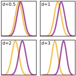 The
value of this comparison between two means becomes clear when we look
at the picture taken from the Wikipedia on the right. Recall that 95%
of values of a normal distribution will fluctuate 2 standard
deviations around the mean (68–95–99.7
rule). The magnitude of the found astrological difference does
matter, but the expected variance does as well. With a small effect
size the estimated means of both groups do not differ that much in
terms of standard deviations. Then most values in both groups, that
will also fluctuate around their mean values, will overlap too. And
for this reason you could not really predict with it. You could only
speculate.
The
value of this comparison between two means becomes clear when we look
at the picture taken from the Wikipedia on the right. Recall that 95%
of values of a normal distribution will fluctuate 2 standard
deviations around the mean (68–95–99.7
rule). The magnitude of the found astrological difference does
matter, but the expected variance does as well. With a small effect
size the estimated means of both groups do not differ that much in
terms of standard deviations. Then most values in both groups, that
will also fluctuate around their mean values, will overlap too. And
for this reason you could not really predict with it. You could only
speculate.
In the case of a small effect with d = 0,2 to 0,5, the differences between the two found means are so small that their normal distributions almost fully overlap. This is the reason why found differences with small effect sizes, are seldom predictive at the individual level. Effect sizes will be low and confidence intervals large, and most group members will overlap with the other group because of variance. Nevertheless, effect size factors of a few percent do influence the profit margins of insurance companies and might also be beneficial to public health, because of the many cases that could for years be exposed to it. A successful campaign against smoking could be an example of it.
Even with a large effects having d=1, there might be some 50% of overlap between the found means of both groups. It is thus still not that predictive at the individual level, but if both groups represented two alternative ways of living, say quitting with smoking or not, many individuals could profit from the positive effect in the long term. But you certainly could not predict the next lottery winner with it.
Only with huge effects when d=2 or larger, most of the found mean values in both groups would not overlap. Here the found differences will also be more predictive at the individual level. The effect of wearing a helmet when sporting could be an example.
The protective effect of wearing a helmet on the WWI battlefield would be quite obvious. So obvious, that you did not need to consult a statistician or astrologer to see the benefit of it. In those cases a cosmic Cohen d-effect could be expected.
When interpreting at the individual level, we cannot rely on large Cohen's d effect sizes, because they deal with the mean difference of groups. They answer major statistical questions like, if any group effect size is seen at all and how large it could be, based on the comparison of the mean values and the variance found in different groups.
But most group members do not behave like their group mean. Actually, the same group members can behave quite differently in different situations. This is the behavioural equivalent of what statisticians call variance. We saw this with the binomial distribution of throwing dices, where the intuitively seen most likely outcomes were statistically seen not that likely at all. And this will even more often happen with astrological questions, because the degrees of freedom involved with a twelve sided dice.
For this reason, few sun signs would fully identify with their sun or moon sign, at least not with its presumed bad habits. And a left wing member of a right wing party, might vote more leftist than most members of a left wing party and vice versa. This normal variation leads to unpredictability. Dictators do not like it and try to get rid of dissidents. Others people ignore the found diversity, leading to cognitive dissonance.
But variation can also be taken into account. So, when confidence intervals are large or effects sizes are small, as was typically found in ADB categories, you cannot predict with it at the individual level. When considering some isolated planets in sign or house, astrologers could only predict and explain events with it at the group level. Only when many small factors point to one direction, the chance of a correct individual prediction or explanation could increase enough enough to do an educated guess.
Astrologers warn against generalisations. But at the same time, they ignore the problem of statistical variation, when they assume that the interpreter has to consider the whole chart, as if it were possible to understand the interaction of all its components. They simply explain away the many exceptions to their rules with supposed to be known other modifying astrological factors, thus with the complexity of the chart, transits and so on.
When a Taurean just by chance displayed Taurean behaviour, biased astrologers would see this as a case for astrology and when he did not, there should be some other astrological factor involved with it. But, astrologers never provided any serious statistical evidence for the presumed effect or interaction of any of them. And that is serious problem. How could a judge ever believe a suspect who explains his incredible statements with other incredible statements?
The problem is that you cannot reasonably explain events afterwards, when you could not predict them with a reasonable amount of certainty before. This simple argument may seem to be rather abstract, so let us explain it with an example dealing with the calculation of the effectiveness of medication.
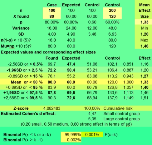 Suppose
we have 80 (out of 100) cures in Treatment Group A and 40
(out of 100) cures in Placebo Group B. The last could be called
spontaneous remissions, and we may reasonably assume that
spontaneous healings will also happen in the treatment group, when
group members were randomly selected.
Suppose
we have 80 (out of 100) cures in Treatment Group A and 40
(out of 100) cures in Placebo Group B. The last could be called
spontaneous remissions, and we may reasonably assume that
spontaneous healings will also happen in the treatment group, when
group members were randomly selected.
The standard deviation (SD) can be estimated as the square root (sqrt) of variance being np(1-p).
For treatment Group A (n=100, p=0,8) the SD is sqrt of (100*0,8(1-0,8)) is sqrt (16) is 4.
For placebo Group B (n=100, p=0,4) the SD is sqrt of (100*0,4(1-0,4)) is sqrt (24) is 4,9.
For both Groups (n=200, p=0,6) the SD is sqrt of (200*0,6(1-0,6)) is sqrt (48) is 6,93.
The pooled SD is sqrt ((16 + 24)/2) = sqrt 20 = 4,47.
From the estimated or better found standard deviations confidence intervals (c.i.) can be estimated. The estimates 99%, 95% and 70% confidence intervals of case and control groups are found in the lower part of the calculator. For the case group with a mean of 80 the 95% ci is 72,2 - 87,8. The expected value based on the findings in both groups has a mean of 60 and a 95% c.i. of 53,21 - 66,79.
In this case the 95% confidence intervals (curves of most likely mean values) do not overlap (Cohen's d is 5,35) and this is a clear indicator of a weak positive effect size (1,33 with a 95% ci of 1,20 - 1,46).
If you measured 80 cures against 53 to 67 expected (mean 60, +/- 7), you would not expect that medicine to be a harmful malefic. The Null hypothesis could be rejected. But there could be questions about the magnitude of its effectiveness. It could be something more or less around the found value, the expected mean np. That something more or less is what statisticians called variance.
Statisticians did many experiments with variance and the square root of it, the standard deviation (SD). They empirically found out that the standard deviation of a sample could predict how often and how far the values of a random sample would deviate from the expected mean value in a normally distributed population. A range of plus / minus one standard deviation (SD) away from the found and most likely mean value could predict the real mean value in 67% of cases and in almost 95% of cases with a value of NP +/- 2 SD.
You find those values under Expected values and corresponding effect sizes in the calculator. With an expected variance of 4 in the treatment group, the 95% confidence interval of the found cure rate of rate of 80% would be 72,2 - 87,8 % (2nd row).
According to the Null hypothesis the cure rate would be the same in the case and control groups. The expected cure rate would then be (80+40) / 200 is 60% with a 95% confidence interval of 53,2 - 66,8 (fourth column). The SD of 6,93 in the control group predicts that the found 120 cures would have a 95% confidence interval of 106,4 - 133,6 (fifth column). This translates to the range of expected values of 53,2 - 66,8 around the mean of 60 in the fourth column. It has a more narrow range than that given in the third column and would result in the higher expected Cohen's d value (5,35 instead of 4,47) when working with large control groups. Because the larger the (control) group, the more accurate the estimation of the group's mean will be (5th lower column). And this accurateness translates into a smaller confidence interval, less overlap between groups and thus a higher Cohen's d value. It would not influence the effect size per se, but would yield a better estimate of it having a smaller range of error (confidence interval).
But with treatment group of 100, we have to deal with the SD of 4,9 of the expected values in the third column. Found values in the treatment group below 50 (50,4) would refer to significant harmful influences (much less cure than expected) and values above 70 (69,6) would imply a significant beneficial effect (much more cures than expected). Found values between 50 and 70 would have insufficient statistical significance to decide that their group means differed enough. Then we deal with a small mean group effect size, that could never be predictive at the individual level at all. Because the found values in both groups would have too much overlap.
The found value of 80 clearly falls outside of the by the Null hypothesis expected range of 50 - 70 cures. Thus the Null hypothesis that both groups are statistically seen the same (only differ because of the sampling error) should be rejected. The effect size would then be 80 against 60 expected is 1,33 with a 95% confidence interval of 1,20 to 1,47 (upper right).
Cohen's d value would be (80-60)/ 4,47 = 4,47 (small control group) or 5,35 (large control group). This is a significant effect that clearly differentiates the results found in both groups. There is no overlap between the found cure rate of 80 % (expected range 72 - 88 %) and the expected cure rate of 60% (expected range 50 - 70%). But though the effect size of 1,33 (1,20-1,47) is significant, it is not that large. For this reason individual outcomes cannot be predicted or being explained with it. That would just be speculation.
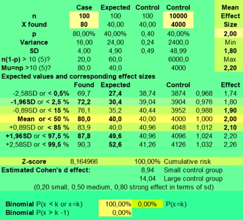 When
filling in n is 10000 and X found is 4000 for the control group, the
effect size of 2,00 (range 1,80 - 2,20) would be seen. Cohen's d
value would be 40/4,47 is 8,94, which is a huge statistical effect
according to this table taken from the Wikipedia page Effect
size.
When
filling in n is 10000 and X found is 4000 for the control group, the
effect size of 2,00 (range 1,80 - 2,20) would be seen. Cohen's d
value would be 40/4,47 is 8,94, which is a huge statistical effect
according to this table taken from the Wikipedia page Effect
size.
|
Effect size |
Cohen's d |
Reference |
|---|---|---|
|
Very small |
0,01 |
Sawilowsky, 2009 |
|
Small |
0,20 |
Cohen, 1988 |
|
Medium |
0,50 |
Cohen, 1988 |
|
Large |
0,80 |
Cohen, 1988 |
|
Very large |
1,20 |
Sawilowsky, 2009 |
|
Huge |
2,00 |
Sawilowsky, 2009 |
And when the spontaneous cure rate of the population was known to be 40% (based on a study of 10.000 cases), we might assume an effect size of 80/40 is 2 (1,8 - 2,2), relating to 72 to 88 % of the 100 patients cured against 40 % (39 - 41) expected.
Cohen's d value would be larger with a large control group B. Here we could take the value 14,04 (large control) for Cohen's d, instead of the value 8,94 for a control group of 100 (small control).
All outcomes are statistically seen huge effects: There would be no discussion about the direction of the effect, as there is minimal overlap with regards to the estimated mean cure rate. So there is knowledge as actionable information you can base your decisions on . But when doing individual predictions, there still will be a lot of uncertainty. Will the treatment work for me? Nobody can tell you. At the individual level, predictions can only be given as possibilities. And explanations of established facts also have to take them into account. In both groups some people are cured (80 + 40 =120) and some are not (20 + 60 = 80). Most often it works with a cure rate of 80% against 40% found for placebo. That can be said.
So one cannot say to an individual person: Oh, you are cured, so you must have had the medicine (this only applies to 80/120 of them), or conclude that the not cured patients must have had placebo (this only applies to 60/80 of them). The same uncertainty exists when you interpret facts afterwards as it does when you had to predict them before. But the last is typically ignored by people who see something that fits their expectations.
In the case of getting 12 times Sun in Taurus out of 79, with a strong Cohen's effect (2,28) there still could be discussion on the existence of any effect: It is 1,75 with an estimated confidence interval of 0,82 - 2,68. So there could be small negative effect (0,82) as well. See this picture above.
 But
if we would have found 790 cases of art critics with 120 of them
having Sun in taurus, having the same mean effect size of 1,75, the
Cohen's d value of 7,19 (large control group) would be huge and there
could be no discussion about its positive effect size (95% confidence
interval 1,46 - 2,04).
But
if we would have found 790 cases of art critics with 120 of them
having Sun in taurus, having the same mean effect size of 1,75, the
Cohen's d value of 7,19 (large control group) would be huge and there
could be no discussion about its positive effect size (95% confidence
interval 1,46 - 2,04).
But it is also obvious that most art critics (85%) do not have Sun in taurus. Could you work with it? No, not very well.
You cannot predict well with small effect sizes, even if reliable studies have been done. And you certainly cannot predict with mistaken astrological assumptions that were never proven to be true. For this reason, astrologers showed up to be bad predictors in most experiments. Even though they could make themselves believe that they still could explain events afterwards.
It became their job to provide meaning to their clients, which was according them something special, statisticians and scientists were not interested in. Of course that assumption was wrong, as statisticians and medical doctors are very concerned with the cancer patients they do research on. But they know that only correct calculations could save life's. So for them the most predictive values count, not the seemingly best hindsight wisdom opportunists make use of.
When studying a random sample of a normally distributed population, we might expect that in 70% of the cases the found value will only fluctuate almost one standard deviation around the mean. In 95% of the cases, found value's would fluctuate +/ - 2 SD around the mean.
If we see an astrological difference in our ADB samples, we might conclude that the selected samples actually did differ in the astrological way. But different samples of the ADB will always be different, because of the sampling error. For this reason we calculated confidence intervals to give significance to the found differences. Could we expect them in a random sample? Or is it unlikely that the found astrological differences just could have been arisen by chance?
We had twelve times Sun in Taurus (75% more) and only two times Sun in Aquarius (70% less often) under art critics. But we also saw that these extreme values still were within the 95% of cases that could be have been arisen just by chance. If the sample size is small, even seemingly large effects are not likely to be statistically significant. And in that case increasing the sample size just might prove the empirical law of regression to the mean. This happens most of the times when doing astrological research.
But what makes a difference large enough? Statistical significance is not all there is. Groups that are different at a 4% or 6% level of significance level do not differ that much. So, for this reason Cohen's d value can act as wise judge. Should we ignore the found differences or not? Negative correlation's are labelled red.
|
Aries |
Taurus |
Gemini |
Cancer |
Leo |
Virgo |
Libra |
Scorpio |
Sag |
Cap |
Aqua |
Pisces |
Total |
|
|---|---|---|---|---|---|---|---|---|---|---|---|---|---|
|
Sun |
1,01 |
2,37 |
0,53 |
1,50 |
1,02 |
-0,68 |
-1,15 |
-0,51 |
-1,39 |
-0,64 |
-2,12 |
0,05 |
-0,00 |
|
Moon |
-0,42 |
1,51 |
-1,01 |
-1,46 |
1,42 |
0,92 |
0,89 |
-2,73 |
0,26 |
0,82 |
1,40 |
-1,60 |
0,00 |
|
Mercury |
1,32 |
0,91 |
2,48 |
-0,00 |
1,83 |
-1,29 |
-1,88 |
0,04 |
-1,46 |
-1,96 |
-1,02 |
1,03 |
0,00 |
|
Venus |
0,52 |
1,16 |
0,26 |
2,53 |
1,70 |
-0,83 |
-0,86 |
-1,40 |
-0,75 |
-0,86 |
-0,76 |
-0,71 |
0,00 |
|
Mars |
2,21 |
-0,11 |
-1,54 |
0,85 |
-2,01 |
1,61 |
-1,26 |
0,57 |
-0,10 |
1,23 |
-1,25 |
-0,19 |
-0,00 |
|
Jupiter |
0,48 |
0,88 |
3,65 |
-1,63 |
0,51 |
-0,18 |
-1,14 |
-0,17 |
0,48 |
-1,53 |
0,01 |
-1,37 |
0,00 |
|
Saturn |
0,78 |
2,13 |
1,38 |
-2,04 |
0,33 |
0,86 |
-0,68 |
-0,76 |
-1,72 |
1,30 |
-2,11 |
0,53 |
-0,00 |
|
Uranus |
0,89 |
1,10 |
-0,52 |
-0,78 |
-0,12 |
-0,01 |
-1,64 |
0,99 |
-2,04 |
1,73 |
0,73 |
-0,33 |
0,00 |
|
Neptune |
1,07 |
1,18 |
0,45 |
1,38 |
-0,37 |
0,54 |
-1,82 |
-1,56 |
-0,85 |
-0,21 |
-0,53 |
0,73 |
0,00 |
|
Pluto |
-0,09 |
1,80 |
0,67 |
0,25 |
-0,99 |
-0,92 |
-0,49 |
-0,11 |
-0,15 |
-0,09 |
0,07 |
0,05 |
0,00 |
|
N Node |
1,07 |
2,09 |
-1,48 |
-1,42 |
-0,30 |
-1,27 |
-0,77 |
1,33 |
-1,05 |
-0,09 |
-0,70 |
2,60 |
0,00 |
|
Chiron |
0,14 |
0,91 |
-1,03 |
0,06 |
0,27 |
-0,15 |
0,43 |
-0,60 |
-0,69 |
-0,33 |
0,51 |
0,47 |
0,00 |
The following table gives the found Cohen's values of the Placidus house cusps.
|
Aries |
Taurus |
Gemini |
Cancer |
Leo |
Virgo |
Libra |
Scorpio |
Sag |
Cap |
Aqua |
Pisces |
Total |
|
|---|---|---|---|---|---|---|---|---|---|---|---|---|---|
|
Cusp 1 |
0,14 |
0,17 |
0,29 |
-1,64 |
0,13 |
0,19 |
-2,34 |
0,67 |
0,07 |
2,05 |
0,15 |
0,14 |
-0,00 |
|
Cusp 2 |
1,01 |
-0,51 |
1,04 |
-0,73 |
-1,23 |
0,13 |
0,48 |
-2,52 |
1,07 |
-1,46 |
2,92 |
-0,19 |
-0,00 |
|
Cusp 3 |
1,61 |
0,64 |
1,27 |
-0,26 |
-1,87 |
-0,62 |
-0,48 |
0,35 |
-2,61 |
0,82 |
-1,65 |
2,81 |
0,00 |
|
Cusp 4 |
1,40 |
2,50 |
1,24 |
0,61 |
-0,45 |
-1,40 |
-0,22 |
-0,31 |
0,56 |
-2,18 |
-1,03 |
-0,71 |
0,00 |
|
Cusp 5 |
-0,99 |
2,14 |
1,44 |
-0,37 |
1,67 |
-0,24 |
-0,74 |
-1,59 |
0,62 |
-0,19 |
-1,29 |
-0,47 |
0,00 |
|
Cusp 6 |
-0,24 |
-1,09 |
2,88 |
1,30 |
-1,17 |
0,52 |
0,55 |
-0,84 |
-0,96 |
0,09 |
0,05 |
-1,08 |
0,00 |
|
Cusp 7 |
-2,34 |
0,67 |
0,07 |
2,05 |
0,15 |
0,14 |
0,14 |
0,17 |
0,29 |
-1,64 |
0,13 |
0,19 |
-0,00 |
|
Cusp 8 |
0,48 |
-2,52 |
1,07 |
-1,46 |
2,92 |
-0,19 |
1,01 |
-0,51 |
1,04 |
-0,73 |
-1,23 |
0,13 |
-0,00 |
|
Cusp 9 |
-0,48 |
0,35 |
-2,61 |
0,82 |
-1,65 |
2,81 |
1,61 |
0,64 |
1,27 |
-0,26 |
-1,87 |
-0,62 |
0,00 |
|
Cusp 10 |
-0,22 |
-0,31 |
0,56 |
-2,18 |
-1,03 |
-0,71 |
1,40 |
2,50 |
1,24 |
0,61 |
-0,45 |
-1,40 |
0,00 |
|
Cusp 11 |
-0,74 |
-1,59 |
0,62 |
-0,19 |
-1,29 |
-0,47 |
-0,99 |
2,14 |
1,44 |
-0,37 |
1,67 |
-0,24 |
-0,00 |
|
Cusp 12 |
0,55 |
-0,84 |
-0,96 |
0,09 |
0,05 |
-1,08 |
-0,24 |
-1,09 |
2,88 |
1,30 |
-1,17 |
0,52 |
0,00 |
We see that the 2-8 axis contains the lowest (-2,52 is very large effect) score for cusp 8 in Taurus (or cusp 2 in Scorpio). The highest positive score (2,92) is largest for cusp 2 in Aquarius and/or cusp 8 in Leo.
For the planets in the houses, Uranus in 7 (3,46) Pluto in 5 (3,13) and Venus in 9 (3,27) have the strong positive effects. Sun in 1 (-2,69), Pluto in 8 (-2,58) would least fit an art critic, being maybe a little bit too intense?
|
H1 |
H2 |
H3 |
H4 |
H5 |
H6 |
H7 |
H8 |
H9 |
H10 |
H11 |
H12 |
Total |
|
|---|---|---|---|---|---|---|---|---|---|---|---|---|---|
|
Sun |
-2,69 |
-0,88 |
0,26 |
-0,12 |
-0,59 |
1,01 |
0,88 |
0,04 |
-0,02 |
2,86 |
-0,31 |
-0,45 |
-0,00 |
|
Moon |
1,84 |
0,77 |
0,72 |
-0,29 |
-1,34 |
1,83 |
-0,90 |
0,29 |
1,82 |
-2,41 |
-0,88 |
-1,43 |
0,00 |
|
Mercury |
-1,73 |
-2,30 |
-0,64 |
0,51 |
0,79 |
0,86 |
-1,28 |
2,31 |
1,14 |
2,24 |
-1,57 |
-0,33 |
-0,00 |
|
Venus |
-0,18 |
0,97 |
0,65 |
-1,55 |
-0,03 |
-0,39 |
-0,42 |
1,51 |
3,27 |
-1,45 |
-1,15 |
-1,23 |
0,00 |
|
Mars |
-0,36 |
-0,32 |
-1,59 |
-1,94 |
0,31 |
0,42 |
2,10 |
2,48 |
-0,24 |
-0,88 |
1,42 |
-1,40 |
0,00 |
|
Jupiter |
-1,34 |
0,19 |
-0,90 |
2,36 |
1,77 |
0,76 |
0,82 |
1,36 |
-0,27 |
-1,49 |
-1,30 |
-1,96 |
0,00 |
|
Saturn |
0,71 |
-0,38 |
-0,28 |
2,42 |
-2,61 |
0,77 |
0,76 |
-0,80 |
0,38 |
1,45 |
-2,03 |
-0,39 |
0,00 |
|
Uranus |
-0,31 |
-1,28 |
0,35 |
-1,33 |
-1,40 |
0,32 |
3,46 |
-0,90 |
0,63 |
1,25 |
-0,47 |
-0,31 |
-0,00 |
|
Neptune |
-1,92 |
-0,26 |
-0,77 |
2,50 |
2,43 |
0,30 |
-1,41 |
-1,00 |
-1,03 |
-0,32 |
1,28 |
0,20 |
-0,00 |
|
Pluto |
-0,89 |
-0,22 |
1,87 |
0,19 |
3,13 |
0,26 |
-0,28 |
-2,58 |
0,20 |
0,25 |
-0,44 |
-1,48 |
0,00 |
|
N Node |
-0,27 |
1,98 |
-2,52 |
-0,29 |
-1,00 |
-0,34 |
-0,85 |
0,28 |
2,98 |
-0,34 |
0,20 |
0,17 |
-0,00 |
|
Chiron |
1,31 |
-0,28 |
1,37 |
-0,82 |
-1,94 |
-1,35 |
2,30 |
1,84 |
-1,94 |
0,16 |
-0,30 |
-0,35 |
0,00 |
The aspects between planets can be studied in the same way a s the other astrological parameters. This is done by quantitatively comparing found and expected values between groups. But statistical conclusions can seldom be done when the expected frequencies are below 10. Here astrologers and statisticians go separate ways. We will try to explain you the reasons why.
Encountering unusual events happens all the time in astrological practice, as every chart and moment in time is unique. But astrologers typically attribute qualitative meaning to coincident events of which statisticians would say that they just could have happened by chance. Statisticians would then leave the topic, stating that much more and larger studies should be done to be able to say anything senseful about that event. But astrologers presume that past astrologers already did this work.
When the horoscope could not that easily explain the natives life or personality according to astrological rules, astrologers would do more studies at the individual level, trying out out different techniques. Like statisticians they prefer to focus on what is essential, so They ignore aspects and other findings that do not fit their big picture. But they would have many objections to discard a great horoscope where most planets and aspects seem to fit their theories as probably just being a random coincidence and thus not statistically significant. On the contrary, they would write an illustrative article about it, as being a great case for astrology that should be studied by all. It would be a prototype, a real archetype, being kicking and alive for them. A great kind of qualitative research that should astonish the skeptics.
But that skeptic scientist could reply with:
Statistician are interested in all the accessible data, not in believe systems just illustrated with some data. The problem is that anyone can base any speculative theory on some cases. But that could at best support hypothesis forming. And in the worst case just framing a story. To make a rule of it one should test the theory by doing enough observations of similar cases using control groups. As you cannot expect that your findings, your particular view on the whole, are representative of a rule. It is only your particular view. Astrologers have to come with much better research.
The judicial principle that who argues proves seems logic and reasonable, but in astrological practice this is seldom seen. What most happens is that shared believes of the astrological tradition, are endlessly repeated on the hand of incidental findings, good story telling, but without reference to any systematic research.
This could lead to endless discussions like this:
Astrologers and statisticians could agree on one thing: The actual risks involved with astronomical events. So let us first try to estimate the probabilities involved with aspects between planets. Maybe we could at least agree on the the mathematical rules that are involved with it.
Remember that the expected mean frequency of any research is np. If we look for conjunctions of planet A with an orb of 10 degrees, a conjunct planet B must be in a range of 10 degrees before or after planet A.
That risk could be simply calculated as 20/360 degrees is 5,556%, if the two planets moved independently as seen from the earth (geocentric point of view). So if you studied 100 charts, on average 5,56 conjunctions between planet A and planet B could be expected.
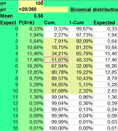 When
would you decide that a found value was outside the expected range
for a certain category? Thus, that this particular aspect is found
much more or less often than expected in a particular group? The kind
of significant astrological findings that should be mentioned in
astrology books.
When
would you decide that a found value was outside the expected range
for a certain category? Thus, that this particular aspect is found
much more or less often than expected in a particular group? The kind
of significant astrological findings that should be mentioned in
astrology books.
Before concluding that a value of 2 or 10 would be quite different from the expected mean value 5 or 6, you should study the binomial distribution for n = 100 and p is 20/360 on the right.
Because we deal with discrete numbers and a skew distribution, the values 5 and 6 are most often found and values from 3 to 7 have an individual risk > 10%. So, it would be risky to base your conclusions on them.
Actually, frequencies from 3 to 7 are statistically seen interchangeable: You could get a 3 or a 7 without knowing that this would be the rule or the exception in the studied population. Because of large confidence interval involved with it. We saw this problem before in the chapter Using the binomial and normal distributions to evaluate frequencies.
Only values of 0, 1, 11 and higher fall outside the in 95% of cases to be expected range. They could hint to real astrological effects, but also to selection bias and other effects. But values from 2 to 10 are statistically seen not that significant, even if that range could imply large effect sizes (0,2-2). They are labelled yellow in the picture on the right.
The good news for astrology students is that you can skip the interpretation of the many not that large effect sizes in the by us presented tables of aspects between 12 planets. As most, except the extreme values, would just fall in the not being that statistically significant range. To help you decide which one's are not to skipped requires some calculations. We will provide a table for this later.
The bad news for astrology students is that you really must do a lot of studies with very large groups and control groups, before you can conclude you understand the effects of aspects. And I do not expect that any famous astrologer with a lot of experience ever did them. And if they actually did them, they just forgot to report the found effects sizes and their confidence intervals.
Astrological rules seem very logic and simple when being explained in astrology books, but that is just the art of framing the astrological theory. The Jesus story was also repeated very successfully, but still belongs to the realm of mythology. In practice we did not find back the strong astrological effects suggested in astrology books.
In our study the measured aspects between planets and their orbs were:
|
conjunction |
6 |
trine |
6 |
|
semi_sextile |
2 |
sesquiquadrate |
2 |
|
semi_square |
2 |
biquintile |
2 |
|
sextile |
4 |
quincunx |
2 |
|
quintile |
2 |
opposite |
6 |
|
square |
6 |
The orbs of the major aspects were set rather narrow to avoid overlap between aspects. And also because one can explain everything one wants, when using large orbs. For this reason rectifiers do not use them. But small orbs of 1 or less were also avoided, as you really need very large study groups to find enough cases of them.
The ADB Research Group provides comparison groups with several orbs. See: Control groups. They can be used for more advanced study of aspects.
The theoretical risk for a square, trine or lesser aspect is twice that of a conjunction or opposition for geometrical reasons. Per degree on the circle, you can have a square by adding 90 degrees or subtracting 90 degrees. The same applies to a trine and the minor aspects. But when you added or subtracted 0 (conjunction) or 180 degrees (opposition), you would arrive at the same point on the circle.
The theoretical risk of getting a trine or square using an orb of 6 is 6*2*2 / 360 = 24 / 360 = 6,67% and the expected value np is 24*79/360 is 5,26 in our study group.
The theoretical formula for the expected value of any left or right dual aspect is: Twice the orb to get the range of degrees * (times) 2 for left and right sided variants * (times) n (sample size) / (divided by) the 360 degrees of the circle.
But there are exceptions to this rule, as the planets do not move as independent factors at the same speed around the by us used Western (not sidereal) zodiac. For this reason we used in all of our calculations the adb_export_181128_2309 export file with n is 55047 as a control group.
For instance look at this Table with expected frequencies of conjunctions between planets using an orb of orb 6 degrees for our sample size of 79. They are based on the adb_export_181128_2309 export control group with n is 55047. The expected values are thus based on empirical findings, not on theoretical considerations.
|
Conjunction: Orb Factor: +- 6 |
|||||||||||
|
Sun |
|||||||||||
|
2,60 |
Moon |
||||||||||
|
13,53 |
2,66 |
Mercury |
|||||||||
|
7,31 |
2,51 |
7,98 |
Venus |
||||||||
|
4,38 |
2,62 |
4,72 |
4,48 |
Mars |
|||||||
|
3,13 |
2,59 |
3,19 |
3,16 |
2,74 |
Jupiter |
||||||
|
2,99 |
2,59 |
2,96 |
2,83 |
3,01 |
2,67 |
Saturn |
|||||
|
2,89 |
2,54 |
2,84 |
2,81 |
2,78 |
3,29 |
2,56 |
Uranus |
||||
|
2,74 |
2,67 |
2,68 |
2,75 |
2,72 |
2,76 |
2,43 |
1,48 |
Neptune |
|||
|
2,77 |
2,62 |
2,68 |
2,64 |
2,70 |
2,56 |
2,92 |
3,17 |
3,31 |
Pluto |
||
|
2,75 |
2,70 |
2,52 |
2,77 |
2,65 |
2,25 |
2,19 |
2,35 |
2,53 |
2,43 |
N Node |
|
|
2,90 |
2,74 |
2,69 |
3,05 |
2,15 |
3,87 |
1,37 |
0,85 |
2,61 |
2,22 |
2,60 |
Chiron |
As you can see most values are near the expected value 79*2*6/360 = 2,63, which would in the binomial practice of discrete numbers be 2 (25,16%) or 3 (22,16%). But, as we could expect, only the found values of the fast moving moon were closest to the calculated mean of 2,63.
The inner planets, being always close to the Sun, will of course much more often have conjunction with the sun and each other. They will never have an opposition or even a trine to the Sun as you can see in the tables of expected values.
Sun Mars conjunctions were found 4,38 / 2,63 is 1,66 times more often than expected, whilst oppositions were found in 0,91 cases against 2,63 expected. An article of the NASA (*) explains this phenomenon with the elliptical orbits of both planets.
During a Sun Mars opposition Mars and the Earth are near to each on the same side of the Sun, so the relative movement of Mars in zodiacal degrees per day is maximal. During a Sun Mars conjunction, Mars is most far away from the Earth, so it seems to move more slowly along the Zodiac, resulting in a longer duration of the conjunction.
For conjunctions between Mars and the inner planets, being always near the Sun, the same mechanism is likely to apply. But we also found a raised conjunction / opposition ratio for the Sun and inner planets with Jupiter and Saturn, though being of a lesser magnitude.
For conjunctions between slow planets, both astronomical factors and the uneven distribution of the ADB control group matters. Because of their slow movement in time, slow planets reflect Zeitgeist and thus certain professions like soldiers will pop up more often than expected in certain times. But dealing with that would be an object of study of cultural history or mundane astrology, we do not understand enough to be able to correct for it.
The next table shows you the Conjunction / Opposition ratio of the whole ADB control group using an orb of 6 degrees.
|
Sun |
|||||||||||
|
0,98 |
Moon |
||||||||||
|
- |
1,01 |
Mercury |
|||||||||
|
- |
0,97 |
- |
Venus |
||||||||
|
4,8 |
0,99 |
5,09 |
4,41 |
Mars |
|||||||
|
1,45 |
1,03 |
1,59 |
1,51 |
1,05 |
Jupiter |
||||||
|
1,25 |
1 |
1,26 |
1,18 |
1,03 |
1,13 |
Saturn |
|||||
|
1,16 |
0,97 |
1,17 |
1,13 |
1,2 |
1,16 |
1,1 |
Uranus |
||||
|
1,05 |
1,03 |
1,06 |
1,07 |
1,11 |
1,05 |
1 |
0,42 |
Neptune |
|||
|
1,17 |
0,98 |
1,03 |
1,03 |
1,12 |
1 |
1,09 |
1,84 |
92,12 |
Pluto |
||
|
0,95 |
1,02 |
0,79 |
1,01 |
0,95 |
0,96 |
0,74 |
0,81 |
1,03 |
1,04 |
N Node |
|
|
1,21 |
1,05 |
1,19 |
1,27 |
1,29 |
1,42 |
0,52 |
0,08 |
2,22 |
0,47 |
0,95 |
Chiron |
Sun Mercury, Sun Venus and Mercury Venus oppositions did not occur for obvious reasons.
For the aspect Sun conjunct Saturn , the from the control group derived expected value with an orb of 6 degrees is 2,99, and can be rounded to 3. It is larger than the theoretical calculated value of 2,63, but this might be an example where the ADB differs from the rest of the population.
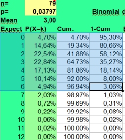 To
find the expected value for 2,63 for an opposition or conjunction,
you simply fill in n =79 and p = 2*6 /360 = +12/360 = 0,03333 in the
binomial calculator. But because we did not know the actual
properties of the world population, we used the expected values
derived from the ADB as a control group.
To
find the expected value for 2,63 for an opposition or conjunction,
you simply fill in n =79 and p = 2*6 /360 = +12/360 = 0,03333 in the
binomial calculator. But because we did not know the actual
properties of the world population, we used the expected values
derived from the ADB as a control group.
What range of frequencies could be expected for Sun conjunct Saturn (expected ADB mean = 3), when we also did take into account the sampling error?
According to the binomial distribution on the right, frequencies from 0 to 6 can be expected quite often. The value 1 is found in 14,64% of cases and even getting a zero (4,70%) would not be a significant finding. As a value below 2,5% was needed for being statistical significant using a two-sided comparison with an an alpha of 0,05. And the value 7, having the low probability of 2,03%, would still not be significant using the 5% divided by 2 is 2,5% criterion of two sided test, because values of the borderline 7 or higher could still be expected in 3,06% of the cases.
So with an expected value of 3, only found values of 8 and above could be called unlikely using a 5% confidence interval. Getting an incidental frequency of zero, when 3 or 4 (79*0,047) of them were to be expected, does by itself have little statistical significance. But when many more zero scores were found something unusual could be happening.
Somewhat higher or lower than expected scores on aspects could be expected all the times. Only high deviations from the expected mean do matter, if the expected mean frequency is not that high (say below 10). But as expected, exceptions to the rule, do also occur. But they do not happen that often. When having just by accident few aspects in a horoscope, the few aspects remaining should get more importance according to Robert Hand in Horoscope Symbols. It would be interesting to see what is the difference between groups having a horoscope with many versus few planetary aspects. But I am not aware of such an study.
Remember that statisticians and other scientists deal with the habits of groups, not with individual persons or atomic particles. So they base their conclusions on the properties of certain groups, unique persons may or may not belong to. And they could combine the found group effects, when individual persons ot groups belonged to several groups. But before you can predict with it, you need to know what is in the data.
Do the ADB groups really differ? And in what sense? Do several categories have more planet to planet links than expected?
To check this hypothesis you could have a look at the Table of all measured aspects of the different ADB categories.
You can also do this for other categories by studying the calculated ADB stats.
Below you see the Table of expected binomial values and their expectancy ranges (for n=79). The shown values are the expected mean (Expected) and the range of values (range) that fall in the 95% confidence interval around that mean, thus values that you could expect in 95% of cases when just taking a random sample of the ADB. Also presented in this table are the involved risks of getting unexpected low or high borderline values. The borderline low and high scores are placed between brackets under the Expected (range). So only values outside that range should be considered as significant at the 5% level, assuming that a binomial distribution determines their scores.
|
Expected (range) |
needed < 2,5% |
borderline low |
borderline high |
needed < 2,5% |
Remark |
|---|---|---|---|---|---|
|
0,88 (0-3) |
3 (4,64%) |
4 (1,18%) |
Expected value using an orb of 1 for unique events (p = 2*1/360 = 1/180 = 0,0111) |
||
|
1 (0-3) |
3 (7,91%) |
4 (1,82%) |
|||
|
1,76 (0-5) |
5 (3,16%) |
6 (0,84%) |
Expected value using an orb of 2 ( p = 2*2*2/360 = 1/45 = 0,0222) |
||
|
2 (0-5 ) |
0 (13,19%) |
5 (5,03%) |
6 (1,52%) |
||
|
2,63 (0-6) |
0 (6,87%) |
6 (4,85%) |
7 (1,64%) |
Conjunctions and oppositions with orb 6 (p =2*6/360 = 1/30 = 0,0333) |
|
|
3 (0-7) |
0 (4,70%) |
7 (3,06%) |
8 (1,03%) |
||
|
3,51 () |
0 (2,76%) |
7 (6,18%) |
8 (2,41%) |
Sextiles with an orb of 4 (p = 2*4*2/360 = 0,0444) |
|
|
4 (1-8) |
0 (1,65%) |
1 (8,60%) |
8 (4,65%) |
9 (1,84%) |
|
|
5 (1-10) |
0 (0,57%) |
1 (3,62%) |
10 (2,72%) |
11 (1,09%) |
|
|
5,27 (1-10) |
0 (0,043%) |
1 (2,85%) |
10 (3,70%) |
11 (1,56%) |
Larger (trines, squares) aspects with an orb 6 (p = 2*6*2/360 = 1/15 = 0,0666) |
|
6 (2-11) |
1 (1,46%) |
2 (5,52%) |
11 (3,63%) |
12 (1,59%) |
|
|
7 (3-12) |
2 (2,48%) |
3 (7,24%) |
12 (4,51%) |
13 (2,12%) |
|
|
8 (3-14) |
2 (1,06%) |
3 (3,52%) |
14 (2,67%) |
15 (1,23%) |
|
|
9 (4-15) |
3 (1,63%) |
4 (4,54%) |
15 (3,21%) |
16 (1,56%) |
|
|
10 (5-16) |
4 (2,23%) |
5 (5,50%) |
16 (3,75%) |
17 (1,89%) |
For an expected value of 10, the range of most likely scores is 5-16 (effect size 0,5 - 1,6). Because we deal with discrete numbers, they contain the borderline low and high frequencies, that do yet fulfil the criterion of being unlikely with an alpha of 0,05. Only discrete values outside that range are expected in less than 5% of cases. So when 10 cases were expected, found values of 4 (effect size 0,40) and below and of 17 (effect size 1,7) or higher would be significant with this sample size.
With an expected value of 5 (range 1-10) only getting a value of 0 or 11 or higher would be statistically seen significant, but values of 1 (effect size 0,2) or 10 (effect size 2) would not be significant at the 5% level, because the risks involved with them would be > 2,5%.
Again: It must be clear that when expected values are low, effect sizes must be quite large, before becoming statistically significant. And here the many In my opinion believers in facts have a problem. Did you really use a control group or did you just suppose you understood what was to be expected? And most important: Did you take the expected variance due to the sampling error into account? As statisticians have good reasons to compare astrology with throwing a 12 sided dice. But astrologers still suppose that this rather random gambling game effect could not apply to the individual chart they studied when they suppose that chance does not exist.
Major aspects (orb 6) with an effect size larger than 2 for the 79 art critics were:
|
Aspect |
x |
exp |
effect |
|---|---|---|---|
|
Sun conjunct Uranus |
8 |
1,34 |
2,92 |
|
Moon conjunct Cheiron |
6 |
2,74 |
2,19 |
|
Mercury conjunct Neptune |
6 |
2,68 |
2,24 |
|
Venus conjunct Jupiter |
7 |
3,16 |
2,21 |
|
Mars conjunct Uranus |
6 |
2,78 |
2,16 |
|
Venus opposite Mars |
4 |
1,02 |
3,93 |
|
Saturn trine Neptune |
10 |
4,99 |
2,00 |
It was tempting to leave out the relatively low score (4 found) of Venus opposite Mars, until we found out that this was a rather unusual constellation. Trines and squares having an effect size larger than 2 were not found, with the exception of Saturn trine Neptune. For trines and squares, also frequencies of 0 could be significant with an expected frequency of 5,27, but they were not found. Trines and squares between the sun and the inner planets were not found in case and control groups.
Aspects between slow planets were not counted, as they chance per generation and we cannot simply use our control group for it.
For small aspects having an orb of 2 the expected frequency is 79 times 8/360 is 1,76 (range 0-5). Because only values of 6 and higher can have statistical significance, found effect sizes should be larger than 3.
Small aspects (orb 2) with an effect size larger the 3 were:
|
Aspect |
x |
exp |
effect |
|---|---|---|---|
|
Mercury semi-sextile Neptune |
6 |
1,86 |
3,22 |
|
Mercury quintile Venus |
3 |
0,76 |
3,97 |
|
Venus quintile Neptune |
6 |
1,78 |
3,37 |
|
Mars biquintile Jupiter |
4 |
1,21 |
3,30 |
|
Jupiter biquintile Saturn |
6 |
1,65 |
3,64 |
Below you see the actually found numbers of All measured aspects between 12 planets found in 79 art critics with the mentioned orbs used.
|
All Aspects |
|||||||||||
|
Sun |
|||||||||||
|
20 |
Moon |
||||||||||
|
11 |
30 |
Mercury |
|||||||||
|
27 |
31 |
24 |
Venus |
||||||||
|
22 |
26 |
35 |
32 |
Mars |
|||||||
|
32 |
32 |
24 |
28 |
31 |
Jupiter |
||||||
|
30 |
25 |
24 |
24 |
26 |
25 |
Saturn |
|||||
|
25 |
30 |
30 |
32 |
35 |
24 |
30 |
Uranus |
||||
|
28 |
32 |
29 |
25 |
25 |
30 |
36 |
34 |
Neptune |
|||
|
26 |
24 |
27 |
23 |
20 |
17 |
26 |
27 |
27 |
Pluto |
||
|
31 |
36 |
28 |
30 |
25 |
33 |
28 |
27 |
29 |
27 |
NorthNode |
|
|
32 |
35 |
35 |
29 |
28 |
31 |
29 |
16 |
31 |
29 |
36 |
Chiron |
In this case the found and expected values are > 10, so calculating effect sizes does make sense.
|
All Aspects |
|||||||||||
|
Sun |
|||||||||||
|
0,67 |
Moon |
||||||||||
|
0,81 |
1,00 |
Mercury |
|||||||||
|
0,91 |
1,04 |
1,01 |
Venus |
||||||||
|
0,77 |
0,87 |
1,22 |
1,10 |
Mars |
|||||||
|
1,08 |
1,08 |
0,80 |
0,95 |
1,05 |
Jupiter |
||||||
|
1,01 |
0,84 |
0,81 |
0,81 |
0,88 |
0,85 |
Saturn |
|||||
|
0,85 |
1,01 |
1,01 |
1,08 |
1,19 |
0,80 |
1,00 |
Uranus |
||||
|
0,94 |
1,07 |
0,97 |
0,84 |
0,85 |
1,02 |
1,21 |
1,10 |
Neptune |
|||
|
0,87 |
0,81 |
0,91 |
0,78 |
0,68 |
0,59 |
0,83 |
0,93 |
0,75 |
Pluto |
||
|
1,05 |
1,20 |
0,96 |
1,01 |
0,86 |
1,12 |
0,91 |
0,93 |
0,96 |
0,92 |
NorthNode |
|
|
1,08 |
1,17 |
1,18 |
0,99 |
0,93 |
0,96 |
1,01 |
0,57 |
0,98 |
1,00 |
1,22 |
Chiron |
But the highest found effect size of 1,22 for Mercury to Mars aspects (35 found against 28,77 expected), is not impressive. The lowest value of 0,67 for Sun and Moon aspects (20 found against 29,9 expected), is also not that strong. One could could not predict with such small effect sizes at the individual level. So they would not be worth to be mentioned in any astrology cookbook, we suppose.
Please also keep in mind, that the most deviating outcomes are just the extremes found in a table of 66 measured aspects, of which on average some 5% or 3,3 found cases, just by chance will deviate from the mean more than expected. And though Sun conjunct Uranus (effect size 2,92) is statistically significant with an alpha of 0,05, it would not be significant any more if we took into account our data mining.
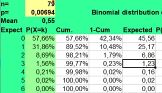 When
dealing with combinations like Sun in the first house AND Sun
in Aries, the separate risks involved with them are multiplied (
multiplication rule). In the most simple astrological model,
we deal with a risk of 1/12 * 1/12 is 1/144 (0,694%).
When
dealing with combinations like Sun in the first house AND Sun
in Aries, the separate risks involved with them are multiplied (
multiplication rule). In the most simple astrological model,
we deal with a risk of 1/12 * 1/12 is 1/144 (0,694%).
The mean expected value np under 79 art critics would then be 79/144 is 0,54861. What does this imply?
According to the binomial distribution on the right, zero frequencies are found most often (58%), a frequency of one would be found in 32% of cases and a two would be expected in 8,7 % of cases. Only values of 3 (1,56%), 4 (0,21% ) and higher (0,02%) are unlikely having an accumulated a risk of 1,79%.
But that does not mean that values of 3 with a risk of 1,56% will not be seen. When studying 79 cases, as we did, one case (np = 1,23) with a frequency of 3 could be expected just by chance. But could you predict with it? Probably not.
For this reason, the author had some reservations to implement these combined calculations in the TkAstroDb. Because unexpected findings will always be found in large contingency tables, but most of them would have little statistical significance. But if unlikely combinations much more often than expected would fit current astrological theories, astrologers could have a case. But is that the case here?
|
Aries |
Taurus |
Gemini |
Cancer |
Leo |
Virgo |
Libra |
Scorpio |
Sag |
Cap |
Aqua |
Pisces |
Total |
||
|
Sun in |
H 1 |
0 |
0 |
1 |
0 |
0 |
1 |
1 |
0 |
0 |
1 |
0 |
0 |
4 |
|
H 2 |
2 |
1 |
0 |
1 |
0 |
0 |
1 |
0 |
1 |
0 |
0 |
0 |
6 |
|
|
H 3 |
1 |
1 |
1 |
1 |
1 |
0 |
0 |
1 |
0 |
1 |
0 |
0 |
7 |
|
|
H 4 |
0 |
1 |
1 |
0 |
1 |
0 |
0 |
1 |
0 |
0 |
0 |
2 |
6 |
|
|
H 5 |
0 |
2 |
0 |
1 |
1 |
0 |
0 |
0 |
0 |
1 |
0 |
0 |
5 |
|
|
H 6 |
1 |
1 |
1 |
2 |
0 |
1 |
1 |
0 |
0 |
0 |
0 |
0 |
7 |
|
|
H 7 |
1 |
1 |
1 |
1 |
2 |
1 |
0 |
0 |
0 |
0 |
0 |
0 |
7 |
|
|
H 8 |
0 |
1 |
0 |
1 |
1 |
0 |
0 |
0 |
2 |
0 |
0 |
1 |
6 |
|
|
H 9 |
1 |
1 |
1 |
0 |
0 |
0 |
1 |
1 |
0 |
0 |
0 |
1 |
6 |
|
|
H 10 |
2 |
3 |
0 |
0 |
2 |
1 |
0 |
2 |
0 |
0 |
1 |
0 |
11 |
|
|
H 11 |
0 |
0 |
1 |
2 |
1 |
0 |
0 |
0 |
0 |
1 |
0 |
2 |
7 |
|
|
H 12 |
1 |
0 |
1 |
1 |
0 |
1 |
0 |
0 |
0 |
1 |
1 |
1 |
7 |
|
|
Total |
9 |
12 |
8 |
10 |
9 |
5 |
4 |
5 |
3 |
5 |
2 |
7 |
79 |
|
If we compare the (theoretical) expected values above with the 144 values actual found under 79 art critics for Sun in Placidus House and sign, we see that in 78 times a zero (54%), 54 times a one (38%), 11 times a two (7,6%) and 1 time a 3 (0,7%) . The actual counts found do not differ that much from the calculated frequencies above using the binomial distribution. Could we attribute meaning to them? Probably not, but a layman not having any understanding of the binomial rules could see something special.
But even statisticians would agree that the finding of 3 (against < 1 expected) found combinations of having Sun in Taurus AND Sun in the 10th house was unusual. They could associate the profession (10th house) art critic with it. So the astrologers could have made a point here.
Statisticians can predict the occurrence of unlikely events, but not where they would occur. At least not under the Null hypothesis. So, when predicting that place before, astrologers could have a case for astrology. Where else did we find particular combinations three or more times? Seven times a value of 4 was found, but this happened only with slow planets.
|
Sun in taurus and H1 Moon in taurus and H9 Moon in virgo and H8 Mercury in aries and H9 Mercury in scorpio and H10 Venus in cancer and H8 Mars in virgo and H9 Mars in sagittarius and H11 Jupiter in taurus and H4 Jupiter in gemini and H8 Jupiter in virgo and H6 Saturn in gemini and H10 Saturn in sagittarius and H12 Saturn in capricorn and H3 |
Uranus in taurus and H7 Uranus in cancer and H7 Uranus in scorpio and H10 Uranus in capricorn and H10 (4 times) Neptune in gemini and H5 (4 times) Neptune in cancer and H4 Pluto in taurus and H4 Pluto in taurus and H5 (4 times) Pluto in taurus and H6 Pluto in taurus and H12 Pluto in gemini and H3 Pluto in gemini and H5 (4 times) Pluto in gemini and H11 (4 times) Pluto in cancer and H3 |
Pluto in cancer and H4 Pluto in cancer and H9 Pluto in cancer and H10 North Node in aries and H2 North Node in taurus and H1 North Node in pisces and H2 (4 times) North Node in pisces and H9 Chiron in aries and H8 Chiron in aries and H12 Chiron in taurus and H4 Chiron in taurus and H10 Chiron in aquarius and H3 Chiron in pisces and H1 (4 times) |
If we put the found >2 values in a diagram, we see that planets in Taurus (12) score best, Leo and Libra score worst with 0.
|
Aries |
Taurus |
Gemini |
Cancer |
Leo |
Virgo |
Libra |
Scorpio |
Sag |
Cap |
Aqua |
Pisces |
|
|
H1 |
Sun NN |
Chiron |
||||||||||
|
H2 |
NN |
NN |
||||||||||
|
H3 |
Pluto |
Pluto |
Saturn |
Chiron |
||||||||
|
H4 |
Jupiter Pluto Chiron |
Neptune Pluto |
||||||||||
|
H5 |
Pluto |
Neptune Pluto |
||||||||||
|
H6 |
Pluto |
Jupiter |
||||||||||
|
H7 |
Uranus |
Uranus |
||||||||||
|
H8 |
Chiron |
Jupiter |
Moon |
|||||||||
|
H9 |
Merc |
Moon |
Venus Pluto |
Mars |
NN |
|||||||
|
H10 |
Saturn Chiron |
Pluto |
Merc, Uranus |
Uranus |
||||||||
|
H11 |
Pluto |
Mars |
||||||||||
|
H12 |
Chiron |
Pluto |
Saturn |
If we would only position slow planets having a found frequency of 4 in the table, we would correct somehow for the uneven distribution of the slow planets in the ADB. Here are the most important planet in house positions of 79 art critics.
|
Aries |
Taurus |
Gemini |
Cancer |
Leo |
Virgo |
Libra |
Scorpio |
Sag |
Cap |
Aqua |
Pisces |
|
|
H1 |
Sun |
Chiron |
||||||||||
|
H2 |
NN |
|||||||||||
|
H3 |
Saturn |
|||||||||||
|
H4 |
Jupiter |
|||||||||||
|
H5 |
Pluto |
Pluto |
||||||||||
|
H6 |
Jupiter |
|||||||||||
|
H7 |
||||||||||||
|
H8 |
Jupiter |
Moon |
||||||||||
|
H9 |
Mercury |
Moon |
Venus |
Mars |
||||||||
|
H10 |
Saturn |
Mercury |
Uranus |
|||||||||
|
H11 |
Pluto |
Mars |
||||||||||
|
H12 |
Saturn |
To be honest, I can make little sense of this statistical profile of being an art critic. And the problem is that with another sample of art critics all the presumed effects could be gone.
According to most astrologers, the ruler (lord) of the first house is very important. When having the cusp of the 1 th house (ascendant) in cancer, the Moon is the so-called chart ruler.
If that Moon is in the 7th House (Lord 1 in House 7 or Lord I in VII), then it is believed that first house affairs (appearance, persona) influence or serve seventh house affairs like partnerships and contracts. So in the case of Donald Trump, having ascendant in Leo ruled by a virgo Sun in House 10 (Lord I in X), his flamboyant Leo persona was a means to bring him to presidency (status, a 10th house affair). Indeed, there could be some truth in it, but we lack enough similar cases to make an astrological rule of it.
In our study of art critics, the signs of the Placidus house cups on the 2-8 axis showed the highest variation, which also showed statistical significance at the 5% level ( X^2= 21,4, p is 0,029). That observation seems to make sense for art critics, as the 2nd house is associated with creating, possessing as well as appreciating things of worth (creating the impulse of aries, having and valuing) and the opposite 8th house with probing values and things in depth with the purpose of alchemy to get rid of the unneeded to start something new (transformation). And that process of creating, destroying and rebuilding heroes and icons of art is of course the core business of art critics.
But that the 2-8 axis is involved does not imply that Taurus and Scorpio should be prominent on those house cusps. As signs are not the same as houses. Actually, the reverse was found: The combination of Cusp 2 in Scorpio and Cusp 8 in Taurus scored four times less than expected (effect size 0,25), whilst the combination Cusp 2 in Aquarius and Cusp 8 in Leo scored highest (2,40 times expected).
|
Aries |
Taurus |
Gemini |
Cancer |
Leo |
Virgo |
Libra |
Scorpio |
Sag |
Cap |
Aqua |
Pisces |
Total |
|
|
Cusp 2 |
1,53 |
0,76 |
1,38 |
0,77 |
0,63 |
1,04 |
1,15 |
0,25 |
1,35 |
0,46 |
2,40 |
0,90 |
12,62 |
|
Cusp 8 |
1,15 |
0,25 |
1,35 |
0,46 |
2,40 |
0,90 |
1,53 |
0,76 |
1,38 |
0,77 |
0,63 |
1,04 |
12,62 |
But scoring much less than expected, can also be a significant finding. But only if the expected frequencies (averages) are high enough to make zero outcomes unlikely. That was not the case when we evaluated aspects. See: What about the aspects?
Notice the symmetry with regards to the cusps in sign frequencies. The cusps axes deal with opposites. Because we used control groups when calculating effect sizes, the effects of slow and fast rising signs were reasonably corrected for.
But now it would be interesting to study the house lords involved with that 2-8 axis. But we will only focus on the most extreme found values, to avoid tasseography based on randomness. See: Using the binomial and normal distributions to evaluate frequencies.
We start with the tables of the modern house rulerships, where 12 planets are assigned to 12 house cusp signs. The research questions is: Do we find unusual high or low scores that fit the idea's of Jean-Baptiste Morin in the context of art critics?
|
Modern House Rulership |
|||||||||||||
|
H 1 |
H 2 |
H 3 |
H 4 |
H 5 |
H 6 |
H 7 |
H 8 |
H 9 |
H 10 |
H 11 |
H 12 |
Total |
|
|
Lord 1 |
4 |
1 |
8 |
8 |
7 |
5 |
11 |
6 |
7 |
10 |
4 |
8 |
79 |
|
Lord 2 |
5 |
6 |
5 |
5 |
7 |
7 |
5 |
8 |
9 |
14 |
2 |
6 |
79 |
|
Lord 3 |
4 |
8 |
5 |
8 |
9 |
5 |
4 |
6 |
10 |
10 |
4 |
6 |
79 |
|
Lord 4 |
6 |
4 |
4 |
6 |
9 |
8 |
8 |
6 |
8 |
4 |
11 |
5 |
79 |
|
Lord 5 |
3 |
5 |
6 |
5 |
5 |
10 |
5 |
9 |
11 |
4 |
9 |
7 |
79 |
|
Lord 6 |
5 |
5 |
6 |
3 |
6 |
13 |
7 |
11 |
7 |
5 |
2 |
9 |
79 |
|
Lord 7 |
8 |
5 |
10 |
6 |
7 |
6 |
7 |
7 |
6 |
6 |
7 |
4 |
79 |
|
Lord 8 |
6 |
6 |
7 |
9 |
8 |
6 |
3 |
5 |
8 |
7 |
9 |
5 |
79 |
|
Lord 9 |
8 |
8 |
5 |
6 |
8 |
9 |
9 |
4 |
4 |
7 |
7 |
4 |
79 |
|
Lord 10 |
6 |
2 |
3 |
7 |
6 |
5 |
6 |
5 |
11 |
11 |
9 |
8 |
79 |
|
Lord 11 |
5 |
4 |
8 |
7 |
12 |
5 |
5 |
5 |
9 |
6 |
5 |
8 |
79 |
|
Lord 12 |
4 |
6 |
9 |
6 |
11 |
8 |
5 |
4 |
8 |
5 |
7 |
6 |
79 |
|
Total |
64 |
60 |
76 |
76 |
95 |
87 |
75 |
76 |
98 |
89 |
76 |
76 |
948 |
When looking at the lords of the second house, we see that Lord 2 in 10 scores 14 (effect size 1,67): creating and valuing things serves the profession. That makes sense. The lowest score is for Lord 2 in 11 (2 found, effect size 0,27), that could point to the fact that art is not for the masses.
When looking at the lords of the eight house, we see no clear winners or losers. The highest value 9 for Lord 8 in 4 (effect size 1,36) and Lord 8 in 11 (effect size 1,27) do not impress. Nor does the lowest value 3 for Lord 8 in 7 (effect size 0,56).
Other high scores were Lord 6 in 6 (13 found, effect size 2,65), which makes sense. The second lowest score was for Lord 6 in 11 (2 found, effect size 0,29)
The chart rulers were most often found in the 7th house (11, effect size 1,57) and 10th house (10, effect size 1,35). House 2 (1, effect size 0,18) scored lowest the house of the chart ruler.
|
Modern House Rulership: Effect sizes |
|||||||||||||
|
H 1 |
H 2 |
H 3 |
H 4 |
H 5 |
H 6 |
H 7 |
H 8 |
H 9 |
H 10 |
H 11 |
H 12 |
Total |
|
|
Lord 1 |
0,73 |
0,18 |
1,41 |
1,30 |
1,09 |
0,79 |
1,57 |
0,78 |
0,84 |
1,35 |
0,60 |
1,27 |
11,91 |
|
Lord 2 |
0,86 |
1,13 |
0,90 |
0,90 |
1,17 |
1,04 |
0,77 |
1,14 |
1,13 |
1,67 |
0,27 |
0,90 |
11,88 |
|
Lord 3 |
0,63 |
1,41 |
0,94 |
1,48 |
1,65 |
0,83 |
0,57 |
0,93 |
1,34 |
1,23 |
0,48 |
0,82 |
12,30 |
|
Lord 4 |
0,86 |
0,67 |
0,73 |
1,15 |
1,68 |
1,42 |
1,20 |
0,84 |
1,17 |
0,54 |
1,33 |
0,62 |
12,22 |
|
Lord 5 |
0,40 |
0,73 |
1,03 |
0,91 |
0,98 |
1,90 |
0,80 |
1,27 |
1,56 |
0,58 |
1,17 |
0,86 |
12,21 |
|
Lord 6 |
0,66 |
0,70 |
0,92 |
0,51 |
1,11 |
2,65 |
1,22 |
1,66 |
0,94 |
0,69 |
0,29 |
1,19 |
12,53 |
|
Lord 7 |
1,08 |
0,71 |
1,47 |
0,97 |
1,15 |
1,11 |
1,35 |
1,17 |
0,84 |
0,80 |
0,98 |
0,57 |
12,18 |
|
Lord 8 |
0,86 |
0,81 |
1,02 |
1,36 |
1,20 |
0,97 |
0,56 |
0,98 |
1,27 |
0,98 |
1,18 |
0,74 |
11,93 |
|
Lord 9 |
1,20 |
1,18 |
0,69 |
0,90 |
1,18 |
1,29 |
1,42 |
0,75 |
0,74 |
1,11 |
0,95 |
0,56 |
11,97 |
|
Lord 10 |
0,93 |
0,29 |
0,44 |
1,03 |
0,92 |
0,77 |
0,77 |
0,83 |
1,94 |
1,90 |
1,33 |
1,13 |
12,28 |
|
Lord 11 |
0,80 |
0,63 |
1,16 |
1,09 |
1,79 |
0,79 |
0,64 |
0,66 |
1,48 |
1,03 |
0,84 |
1,19 |
12,09 |
|
Lord 12 |
0,66 |
1,04 |
1,42 |
0,91 |
1,70 |
1,18 |
0,70 |
0,49 |
1,10 |
0,78 |
1,15 |
1,00 |
12,14 |
|
Total |
9,69 |
9,48 |
12,12 |
12,52 |
15,62 |
14,74 |
11,56 |
11,50 |
14,34 |
12,64 |
10,58 |
10,84 |
145,64 |
When looking at both tables, the column totals suggest that the house rulers were most often found in the fifth house (10% against 8,3% expected).
Here are the corresponding Cohen's d values.
|
Modern House Rulership: Cohen's d values |
|||||||||||||
|
H1 |
H2 |
H3 |
H4 |
H5 |
H6 |
H7 |
H8 |
H9 |
H10 |
H11 |
H12 |
Total |
|
|
Lord 1 |
-0,72 |
-2,23 |
1,13 |
0,90 |
0,27 |
-0,65 |
1,95 |
-0,82 |
-0,64 |
1,25 |
-1,27 |
0,82 |
0,00 |
|
Lord 2 |
-0,37 |
0,31 |
-0,25 |
-0,24 |
0,47 |
0,13 |
-0,70 |
0,45 |
0,46 |
2,56 |
-2,51 |
-0,32 |
0,00 |
|
Lord 3 |
-1,31 |
1,30 |
-0,19 |
1,45 |
1,97 |
-0,55 |
-1,71 |
-0,26 |
1,39 |
1,02 |
-2,36 |
-0,75 |
0,00 |
|
Lord 4 |
-0,56 |
-1,12 |
-0,83 |
0,46 |
2,08 |
1,35 |
0,77 |
-0,66 |
0,68 |
-1,97 |
1,57 |
-1,77 |
0,00 |
|
Lord 5 |
-2,29 |
-0,93 |
0,09 |
-0,24 |
-0,04 |
2,42 |
-0,63 |
0,99 |
2,01 |
-1,48 |
0,69 |
-0,58 |
0,00 |
|
Lord 6 |
-1,10 |
-0,93 |
-0,23 |
-1,23 |
0,25 |
3,50 |
0,55 |
1,88 |
-0,20 |
-0,96 |
-2,14 |
0,61 |
0,00 |
|
Lord 7 |
0,50 |
-1,71 |
2,66 |
-0,18 |
0,77 |
0,48 |
1,50 |
0,85 |
-0,98 |
-1,27 |
-0,09 |
-2,51 |
0,00 |
|
Lord 8 |
-0,69 |
-1,02 |
0,08 |
1,73 |
0,96 |
-0,12 |
-1,75 |
-0,06 |
1,23 |
-0,10 |
1,01 |
-1,28 |
0,00 |
|
Lord 9 |
0,94 |
0,87 |
-1,60 |
-0,47 |
0,85 |
1,43 |
1,84 |
-0,94 |
-0,99 |
0,46 |
-0,24 |
-2,14 |
0,00 |
|
Lord 10 |
-0,21 |
-2,38 |
-1,86 |
0,09 |
-0,27 |
-0,72 |
-0,88 |
-0,52 |
2,63 |
2,56 |
1,10 |
0,45 |
0,00 |
|
Lord 11 |
-0,72 |
-1,42 |
0,65 |
0,35 |
3,14 |
-0,80 |
-1,69 |
-1,49 |
1,73 |
0,09 |
-0,58 |
0,74 |
0,00 |
|
Lord 12 |
-1,31 |
0,14 |
1,71 |
-0,37 |
2,90 |
0,77 |
-1,35 |
-2,65 |
0,47 |
-0,89 |
0,57 |
0,02 |
-0,00 |
|
Total |
-7,84 |
-9,12 |
1,36 |
2,24 |
13,36 |
7,24 |
-2,11 |
-3,23 |
7,80 |
1,28 |
-4,26 |
-6,71 |
-0,00 |
Here are the counts fo r the Traditional House Rulership method:
|
Traditional House Rulership |
||||||||||||||
|
H 1 |
H 2 |
H 3 |
H 4 |
H 5 |
H 6 |
H 7 |
H 8 |
H 9 |
H 10 |
H 11 |
H 12 |
Total |
||
|
Lord 1 |
7 |
6 |
3 |
4 |
10 |
5 |
10 |
8 |
6 |
7 |
5 |
8 |
79 |
|
|
Lord 2 |
7 |
5 |
4 |
6 |
7 |
5 |
6 |
9 |
8 |
12 |
1 |
9 |
79 |
|
|
Lord 3 |
7 |
8 |
7 |
7 |
9 |
5 |
5 |
7 |
6 |
5 |
7 |
6 |
79 |
|
|
Lord 4 |
7 |
6 |
10 |
4 |
5 |
6 |
5 |
9 |
11 |
4 |
9 |
3 |
79 |
|
|
Lord 5 |
2 |
5 |
5 |
7 |
8 |
7 |
4 |
13 |
8 |
9 |
7 |
4 |
79 |
|
|
Lord 6 |
4 |
6 |
5 |
7 |
7 |
9 |
6 |
10 |
7 |
6 |
6 |
6 |
79 |
|
|
Lord 7 |
6 |
7 |
11 |
5 |
8 |
7 |
6 |
11 |
7 |
7 |
3 |
1 |
79 |
|
|
Lord 8 |
4 |
6 |
4 |
9 |
8 |
9 |
6 |
10 |
6 |
6 |
4 |
7 |
79 |
|
|
Lord 9 |
8 |
8 |
4 |
6 |
5 |
10 |
11 |
7 |
5 |
8 |
3 |
4 |
79 |
|
|
Lord 10 |
7 |
5 |
3 |
10 |
1 |
11 |
9 |
5 |
9 |
7 |
6 |
6 |
79 |
|
|
Lord 11 |
9 |
4 |
2 |
10 |
4 |
7 |
9 |
8 |
13 |
3 |
6 |
4 |
79 |
|
|
Lord 12 |
5 |
8 |
5 |
6 |
7 |
8 |
6 |
9 |
9 |
4 |
9 |
3 |
79 |
|
|
Total |
73 |
74 |
63 |
81 |
79 |
89 |
83 |
106 |
95 |
78 |
66 |
61 |
948 |
|
The chart rulers were found most often in the 5th house (10 found, effect size 1,65) dealing with creativity and 7th house (10 found, effect size 1,55) dealing with partnerships.
The tenth house scores best as ruler of the 2nd house (12 found, effect size 1,66). That makes sense as the 10th house is associated with profession and public role. Morinus would say: Valuing things is a means to do the work of art critic. Lord 2 in 8 scores second best score (9 found, effect size 1,40) and also fits. Valuing things is a means to get rid of the crap. As an art critic has to promote art of eternal value. The lowest score if for Lord 2 in House 11 (1 found, 0,14 times as expected): Valuing things is not a way to keep friends, it seems. But that would not surprise us, as art criticism is a rather subjective process.
Nevertheless, the highest scoring chart rulers were in the 5th house (10 found, effect size 1,65) dealing with creativity and 7th house (10 found, effect size 1,55) dealing with partnerships. The lowest value was found for Lord 1 in 3 (3 found, effect size 0,48).
Lord 8 in 8 scores best as the ruler of the eight house under art critics (10 found, effect size 1,71). This could be a destructive variant of l'art pour l'art. The second best is Lord 8 in 6 (9 found, effect size 1,42),which would refer to the daily routine of the art critic. Lord 8 in 4 was also found 9 times, but has a lower effect size (1,34) because of the uneven Placidus houses and other effects.
Here are the effect sizes bases of found values under art critics, as compared to the expected values in the ADB.
|
Traditional House Rulership: Effect sizes |
|||||||||||||
|
H 1 |
H 2 |
H 3 |
H 4 |
H 5 |
H 6 |
H 7 |
H 8 |
H 9 |
H 10 |
H 11 |
H 12 |
Total |
|
|
Lord 1 |
1,05 |
0,91 |
0,48 |
0,66 |
1,65 |
0,83 |
1,55 |
1,27 |
0,89 |
0,95 |
0,69 |
1,11 |
12,04 |
|
Lord 2 |
0,98 |
0,76 |
0,62 |
1,01 |
1,18 |
0,82 |
0,96 |
1,40 |
1,22 |
1,66 |
0,14 |
1,23 |
11,99 |
|
Lord 3 |
0,97 |
1,16 |
1,09 |
1,13 |
1,54 |
0,84 |
0,82 |
1,13 |
0,90 |
0,71 |
0,96 |
0,82 |
12,08 |
|
Lord 4 |
1,00 |
0,88 |
1,49 |
0,64 |
0,81 |
1,02 |
0,82 |
1,46 |
1,75 |
0,57 |
1,24 |
0,41 |
12,09 |
|
Lord 5 |
0,28 |
0,71 |
0,75 |
1,09 |
1,31 |
1,16 |
0,65 |
2,15 |
1,25 |
1,33 |
0,98 |
0,56 |
12,22 |
|
Lord 6 |
0,57 |
0,84 |
0,75 |
1,09 |
1,07 |
1,49 |
0,98 |
1,68 |
1,13 |
0,89 |
0,88 |
0,83 |
12,19 |
|
Lord 7 |
0,83 |
1,00 |
1,60 |
0,77 |
1,22 |
1,09 |
0,98 |
1,78 |
1,15 |
1,07 |
0,45 |
0,15 |
12,09 |
|
Lord 8 |
0,57 |
0,82 |
0,60 |
1,34 |
1,20 |
1,42 |
0,95 |
1,71 |
0,94 |
0,93 |
0,61 |
1,04 |
12,13 |
|
Lord 9 |
1,17 |
1,18 |
0,58 |
0,92 |
0,76 |
1,54 |
1,73 |
1,12 |
0,80 |
1,23 |
0,45 |
0,58 |
12,06 |
|
Lord 10 |
1,05 |
0,73 |
0,45 |
1,50 |
0,16 |
1,74 |
1,36 |
0,79 |
1,38 |
1,06 |
0,88 |
0,89 |
11,99 |
|
Lord 11 |
1,39 |
0,60 |
0,30 |
1,60 |
0,63 |
1,11 |
1,39 |
1,21 |
1,99 |
0,44 |
0,88 |
0,57 |
12,10 |
|
Lord 12 |
0,73 |
1,25 |
0,79 |
0,94 |
1,15 |
1,25 |
0,95 |
1,35 |
1,33 |
0,57 |
1,29 |
0,44 |
12,04 |
|
Total |
10,59 |
10,85 |
9,51 |
12,69 |
12,66 |
14,32 |
13,14 |
17,05 |
14,72 |
11,42 |
9,45 |
8,63 |
145,03 |
As expected they fluctuate around the expected mean of 1 (no effect). The highest values are for Lord 5 in 8 (2,15). The lowest for Lord 12 in 7 (0,15), Lord 10 in 5 (0,16) Lord 5 in 1 (0,28) and Lord 11 in 3 (0,30). Negative effect sizes tend to be stronger, but this could just be a result of skewness of the binomial distribution and our method of determining effect sizes. With larger samples that effect should diminish.
The corresponding Cohen's d value's fluctuate between 3,38 for Lord 5 in 8 to -13,46 for Lord 7 in 12.
|
Traditional House Rulership: Cohen's d values |
|||||||||||||
|
H1 |
H2 |
H3 |
H4 |
H5 |
H6 |
H7 |
H8 |
H9 |
H10 |
H11 |
H12 |
Total |
|
|
Lord 1 |
0,21 |
-0,39 |
-2,07 |
-1,31 |
2,48 |
-0,63 |
2,24 |
1,08 |
-0,48 |
-0,22 |
-1,42 |
0,50 |
0,00 |
|
Lord 2 |
-0,05 |
-0,79 |
-1,20 |
0,04 |
0,52 |
-0,54 |
-0,14 |
1,28 |
0,72 |
2,37 |
-3,04 |
0,84 |
0,00 |
|
Lord 3 |
-0,20 |
1,17 |
0,61 |
0,82 |
3,30 |
-0,98 |
-1,17 |
0,85 |
-0,67 |
-2,09 |
-0,30 |
-1,35 |
0,00 |
|
Lord 4 |
0,01 |
-0,42 |
1,75 |
-1,20 |
-0,64 |
0,05 |
-0,58 |
1,50 |
2,51 |
-1,63 |
0,93 |
-2,29 |
0,00 |
|
Lord 5 |
-2,48 |
-0,98 |
-0,79 |
0,27 |
0,91 |
0,46 |
-1,03 |
3,38 |
0,79 |
1,08 |
-0,06 |
-1,55 |
0,00 |
|
Lord 6 |
-2,58 |
-0,97 |
-1,37 |
0,48 |
0,37 |
2,50 |
-0,12 |
3,41 |
0,66 |
-0,61 |
-0,71 |
-1,06 |
0,00 |
|
Lord 7 |
-0,62 |
0,00 |
2,04 |
-0,73 |
0,71 |
0,30 |
-0,07 |
2,39 |
0,45 |
0,22 |
-1,80 |
-2,90 |
0,00 |
|
Lord 8 |
-2,03 |
-0,86 |
-1,82 |
1,54 |
0,90 |
1,78 |
-0,19 |
2,79 |
-0,27 |
-0,29 |
-1,74 |
0,18 |
-0,00 |
|
Lord 9 |
0,65 |
0,69 |
-1,66 |
-0,28 |
-0,88 |
1,98 |
2,61 |
0,41 |
-0,71 |
0,84 |
-2,04 |
-1,62 |
0,00 |
|
Lord 10 |
0,17 |
-0,89 |
-1,75 |
1,63 |
-2,55 |
2,27 |
1,16 |
-0,65 |
1,19 |
0,18 |
-0,40 |
-0,36 |
-0,00 |
|
Lord 11 |
1,07 |
-1,14 |
-1,98 |
1,59 |
-1,01 |
0,29 |
1,07 |
0,59 |
2,75 |
-1,63 |
-0,35 |
-1,26 |
0,00 |
|
Lord 12 |
-1,27 |
1,08 |
-0,92 |
-0,26 |
0,61 |
1,09 |
-0,20 |
1,59 |
1,51 |
-2,03 |
1,37 |
-2,58 |
0,00 |
|
Total |
-7,12 |
-3,50 |
-9,14 |
2,59 |
4,72 |
8,57 |
3,59 |
18,63 |
8,46 |
-3,80 |
-9,54 |
-13,46 |
-0,00 |
Again most house rules concerned the eighth house.
Statistical ADB researchers could expect a lot of problems, as well as resistance, when studying categories like art critics documented in the ADB. Both statisticians, scientists and astrologers could have many objections to this practice. Just to name a few:
The arguments could to a certain extent be valid, but there are always two sides of the coin. In the empirical practice it is seldom a matter of this or that, as the facts of life are too manifold to fit in a single logical system. But in polemic discussions dealing with astrology and other beliefs, emotions often prevail, resulting in the pot calling the kettle black games that distract the audience from the found facts and simple conclusions.
Nevertheless, astrologers and scientists could agree that statistical information from the ADB still provides better evidence for any case of astrology, than the opinions found in astrology books and forums. As the last more reflect the by astrologers shared idea's and personal speculations than the actual astrological facts. And with a much more improved assignment of categories, the ADB could be the shining diamond of astrology.
Doing better predictions in astrological practice was the goal of the astrologer and data collector Louis Rodden, who set up the ADB. She believed that astrological practice should at last be based on quantitative research and not on the usual speculations found in astrology books. Indeed, astrology students cannot expect to become wise by just studying astrological symbolism as explained to them in astrology books. They also need to process available astrological data in a critical way. And after seeing several point of views and lot of data, then they could try to understand the events in their and others life's.
The process of inner growth is often seen as the purpose of astrology. But, it would be a bad idea to base spiritual growth on false idea's and biased thinking. Even if the idea's were massively shared in your astrology group and you feel happy with it. Books and views that once inspired people to look above to see new horizons, might at other times become a procrustean bed that hampers spiritual growth. A modern theologian cannot grow if he takes the messages of the Bible too literally. And a medical astrologer cannot grow if he sticks to the now obsolete believes of William Lilly or Nicholas Culpeper. As we live in different times. In our article The wisdom hierarchy some consequences of that for astrology are explored.
The qualitative approach, especially that of astrological symbolism, is easy to learn, flexible to use, amusing and exciting, but has no predictive value. Explanations done with it can look very powerful, but what astrologers call the synthesis of the complex chart to come to the essence of it, too often resembles the process of framing :
The quantitative approach is a not that easy to learn, amusing and exciting as the above method. But it suffers less from selective attention and can be really predictive when large case and control groups are used. Using statistical analytical methods, you can even predict when you can and when you cannot predict with it! And that great feature could spare you a lot of time. No need to speculate, no need to procrastinate at night.
When astrology books use vague terms as could or might to hint to expected correlation's between the above and below, they could and should be replaced with more predictive effect sizes and confidence intervals. Then the actual found data and effect sizes could be rather comforting when confronted with your supposed to be difficult Pluto transit. But the method is not that easy to learn, the research is more time consuming and the results can be disappointing.
Nevertheless, with a little basic understanding of statistics and probability calculation, the study of astrology can be a joyful science when you have access to relevant data. Then you could simply check which astrological claims could be true and which claims are probably wrong. You can even estimate confidence intervals with the tools and data we provided.
Notice that the quantitative approach does not exclude qualitative and even symbolic ways of thinking. It only restricts them somewhat, as it requires that claims and questions should be clearly formulated and documented.
When doing astrological research with Radix 5 or TkAstroDb, possible astrological effects that were significant at the 0,05 alpha level tended to be small. And they typically became smaller with a larger sample size. This regression to the mean certainly pleads against astrology as a predictive and explanatory science. When the found astrological effects are too small to predict with, or confidence intervals of supposed to be large effects are wide to rely on, no reasonable interpretation of a single chart could be made with them. As you cannot explain events, that you could not foresee before.
Differences of a few percent might benefit insurance companies dealing with large numbers. And small differences will be relevant in elections, where every vote counts. In that case the winner takes it all. But it is impossible to base astrological consultations on small astrological effects even when the effects and interactions of the many astrological indicators in the chart were actually known. Then a computer supplied with enough relevant data could do calculations to predict or explain things with confidence intervals instead of the usual my two-penny worth astrological speculations.
Gauquelins's plead for neo-astrology based on empirically established astrological rules had few followers under astrologers. As they feared the consequence that most of their astrology books and certificates should be thrown away as being outdated. Astrologers have little understanding of statistical methods, because it contrasts so much with their paradigm that chance does not exist. So they do not feel the need to use control groups or to calculate confidence intervals when doing their research. They rely on selected books of experts in the field and on their own experience. So their control groups are in practice implicit ideas about the astrological reality that only exist in their own heads.
But only in the more radical way proposed by neo-astrologers, focussed on fact finding instead of systematic cherry picking to rescue an outdated belief, astrology could become a more predictive science, instead of the questionable ad hoc habit of framing astrological findings afterwards. For this reason we tried to explain with simple probability calculations that you cannot reasonably explain events afterwards that you could not predict before. Because of the logical fallacy that any fool can unreasonably blame anything he wants for any event, including the stars based on wrong premises.
Even the Mars and other effects could be astronomical anomalies based on the geocentric point of view as we saw in the ADB control groups. Anyway, effect sizes of 20% as found by the Gauquelin's, could be too small to predict with at an individual level. If seven indicators with an effect size of 20% all moved in the same direction, like some Mars effect, we could have an increased risk factor of at most 1,2^7 = 3,6. But those strong combined effects are not predictive enough when dealing with unusual events like becoming a scientist. When the incidence is low, like winning the lottery or becoming a famous medical doctor, the astrologer could not rely on finding seven planets standing favourable.
Mediocre effects could guide trivial questions like: Will I marry him or her this year. If that person was of a certain age and had a stable relation with the native, an astrologer could say yes. But what factors would matter? The twinkling eyes of the native asking the question or the twinkling stars in the sky? Astrologers might afterwards believe that they could explain every single fact, making creative use of the many indicators in any horoscope. But how can one interpret found facts if one could not understand and predict them beforehand? How could the interpretations of modern astrologers ever seem to be somehow right? Without doubt the best astrologers base most of their advise on the many not astrological factors they derived from their clients by observing them and listening to their stories.
Because they never use explicit control groups, astrologers regard any horoscope and any native as as special. And that is what the human ego wants to hear: At last somebody noticed me. Astrologers noticed their clients situation and saw it reflected in the stars, without realising that many more scenario's could pop up as well. Nevertheless, small effects can become relevant in the long-term , because of an accumulated effect. This is the case with smoking, when in time and pack-years the risks of the with smoking associated hazards increase. But if a slow planet transit of Pluto or a secondary progression also acts in this long-lasting way, still has to be proven.
Sjoerd Visser
binomial_distribution_for_astrology.ods was the spreadsheet used to do the statistical calculations with.
The most recent findings of the ADB Research Group can be found at ADB stats.
Tip: Download the 7z files and expand them with 7-Zip.
Gebruik van TkAstroDb voor astrologisch onderzoek (always outdated How To for TkAstoDb in Dutch, but still the best you can get in Dutch)
Why Many Scientists Consider Astrology to Be a Pseudoscience (Video by researcher David Cochrane)
How to Conduct Astrology Research: A Course of 25 Tutorial Videos (Video's by astrologer David Cochrane)
Four Humors - And there's the humor of it: Shakespeare and the four humors
Graven in de ADB met TkAstroDb (NVWOA lecture in Dutch)
Help:Category - Astro-Databank
Help:RR - Astro-Databank : The Rodden Rating refers the the reliability of the mentioned source. But Rodden Ratings are not directly linked to astrological precision. Birth Record times noticed by the midwife rounded to a the whole hour get a RR or AA, but the at the minute exact rectified chart by an experienced astrologer only gets a RR of C(aution).
History of statistics : The history of statistics in the modern way is that it originates from the term statistics, found in 1749 in Germany. Although there have been changes to the interpretation of the word over time. The development of statistics is intimately connected on the one hand with the development of sovereign states, particularly European states following the peace of Westphalia (1648); and the other hand with the development of probability theory, which put statistics on a firm theoretical basis (see history of probability).
Mars Opposition | Mars in our Night Sky – NASA’s Mars Exploration Program :
Ten common statistical mistakes to watch out for when writing or reviewing a manuscript
Kurt Vonnegut, Shape of Stories
Waarom maken politici graag gebruik van framing? - Taalcanon